[sampling]曲面上的随机采样问题 #16
Comments
为何不涉及其它维度?因为都是已经解决的问题。 维度为1的曲线上的均匀分布,实际上就是一般说的均匀分布 维度为2的曲面上的均匀分布,实际上就是平面上某一块区域,以二维圆面为例,算法如下: def random_surface():
while True:
x, y = np.random.rand(2) * 2 - 1
if x ** 2 + y ** 2 <= 1:
return x, y
sample = np.array([random_surface() for i in range(1000)])
plt.plot(sample[:, 0], sample[:, 1], '.')
|

曲线上的均匀随机假设曲线的表示是: 第一类曲线积分 算法就是根据上面的方程,找到$x=f(r)$,然后生成随机的r,进而就找到x了。 |
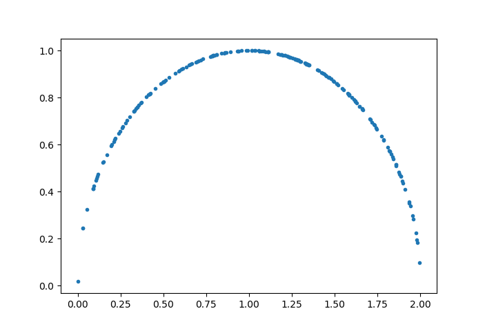
案例:圆
方程是 代码就有了: def random_surface():
r = np.random.rand()
t = r * np.pi
x, y = np.cos(t) + 1, np.sin(t)
return x, y
sample = np.array([random_surface() for i in range(200)])
plt.plot(sample[:, 0], sample[:, 1], '.')
|

缺点与改进以阿基米德螺旋线$x=t\cos t, y=t\sin t$为例, 求积分那一步就已经有点计算量了, import scipy.optimize as opt
import numpy as np
def func(t):
# 被积部分
return np.sqrt(1 + np.square(t))
from scipy import integrate
s, _ = integrate.quad(func, 0, 4 * np.pi) # 分母
result = []
for i in range(300):
# r = np.random.rand()
r = i / 300
t = opt.fsolve(lambda t: integrate.quad(func, 0, t)[0] / s - r, [0], fprime=func)
x = t * np.cos(t)
y = t * np.sin(t)
result.append([x, y])
result = np.array(result)
plt.plot(result[:, 0], result[:, 1], '.')
plt.show()
|

方案3观察到这样的事实,如果把 算法步骤:
代码 import scipy.optimize as opt
import numpy as np
def func(t):
# 被积部分
return np.sqrt(1 + np.square(t))
left, right = 0, 4 * np.pi
m = -opt.minimize(fun=lambda t: -func(t), x0=np.array([0.1]),
method=None, jac=None,
bounds=((left, right),)).fun[0]
t_list = []
for i in range(1000):
t = np.random.rand() * (right - left) + left
if func(t) / m > np.random.rand():
t_list.append(t)
x = t_list * np.cos(t_list)
y = t_list * np.sin(t_list)
plt.plot(x, y, '.')
plt.show()优缺点:
|
|
想了一下,方案3思路是对的,但算法流程是错的。因为归一化时,不应该用 max,而应当用另外一个已知的随机变量去做包洛。 正确的做法是先分段,然后在每段上找一个已知的概率分布去包洛 f(t)。 更正:方案3的算法流程和代码都是对的,因为用max归一化时,之前漏掉的一个因子在后面又被抵消了。使得最后结果还是对的。 不过还没想好如何用绝对均匀的图去验证这个算法 @shouldsee 帮我review一下 |
曲面上的均匀随机推广回到曲线上均匀分布的推导过程,我们找到方程 对于曲面上的情况,类似的, 案例:球面为了符号统一,我们把$f(x,y)$定义在$R^2$上,并且对于原本没有定义的点,定义$f(x,y)=0$ 又记 之后得到$(x',y')$就是我们要的结果 from scipy import optimize as opt
from scipy import integrate
import numpy as np
import matplotlib.pyplot as plt
from mpl_toolkits.mplot3d import Axes3D
fig = plt.figure()
ax = fig.gca(projection='3d')
def bound(x, y):
return x ** 2 + y ** 2 <= 0.9
def func(x, y):
if bound(x, y):
return 1 / np.sqrt(1 - x ** 2 - y ** 2)
else:
return 0
x_min, x_max, y_min, y_max = -0.9, 0.9, -0.9, 0.9
def func_g(x):
g = integrate.quad(lambda y: func(x, y), -np.sqrt(1 - x ** 2), np.sqrt(1 - x ** 2))
return g[0]
# g(x)的最大值
m1 = -opt.minimize(fun=lambda x: -func_g(x), x0=np.array([0.1]),
bounds=((x_min, x_max),)).fun
# f(x,y)的最大值
# m2 = -opt.minimize(fun=lambda xy: -func(xy[0], xy[1]), x0=np.array([0.1, 0.1]),
# bounds=((x_min, x_max), (y_min, y_max))).fun
m2 = np.sqrt(10)
result = []
for i in range(1000):
x = np.random.rand() * (x_max - x_min) + x_min
if func_g(x) / m1 > np.random.rand():
not_find = True
while not_find:
y = np.random.rand() * (y_max - y_min) + y_min
if func(x, y) / m2 > np.random.rand():
result.append([x, y])
not_find = False
# 整理并绘图
result = np.array(result)
X = result[:, 0]
Y = result[:, 1]
Z = np.sqrt(1 - X ** 2 - Y ** 2)
surf = ax.scatter(X, Y, Z)
plt.show()
# %%
np.array([func_g(i) for i in np.arange(-1, 1, 0.1)])
|

|
搞定,虽然warning太多 也就是说,如果某些区域的偏导数太大,算法效率会大大降低。 http://www.guofei.site/2019/08/16/random_surface.html 想到了一个极为美妙的做法,我去写写 |
|
考虑把曲面方程变成参数形式(曲线线的情况就是这么干的)。 假设我们的曲面方程式这个形式 推导过程就不写了,直接上算法流程
以球面为例$\vec r=(\sin u\cos v,\sin u\sin v,\cos u)$ import numpy as np
import scipy.optimize as opt
# 参数方程$r=r(u,v$
def func(u, v):
return np.sin(u) * np.cos(v), np.sin(u) * np.sin(v), np.cos(u)
# r对u的偏导数
def func_r_u(u, v):
return np.cos(u) * np.cos(v), np.cos(u) * np.sin(v), -np.sin(u)
# r对v的偏导数
def func_r_v(u, v):
return -np.sin(u) * np.sin(v), np.sin(u) * np.cos(v), 0
def func_I(u, v):
r_u = func_r_u(u, v)
r_v = func_r_v(u, v)
E = np.linalg.norm(r_u, ord=2)
G = np.linalg.norm(r_v, ord=2)
F = np.dot(r_u, r_v)
return np.sqrt(E * G - F ** 2)
left, right = 0, 2 * np.pi
m = -opt.minimize(fun=lambda t: -func_I(t[0], t[1]), x0=np.array([0.1, 0.1]),
bounds=((left, right), (left, right))).fun
m = m + 0.1
# %%
points = np.random.rand(3000, 2) * np.pi * 2
result = []
for point in points:
if func_I(point[0], point[1]) / m > np.random.rand():
result.append(point)
# %%画图
import matplotlib.pyplot as plt
from mpl_toolkits.mplot3d import Axes3D
fig = plt.figure()
ax = fig.gca(projection='3d')
X, Y, Z = [], [], []
for point in result:
u, v = point
x, y, z = func(u, v)
X.append(x)
Y.append(y)
Z.append(z)
X = np.array(X)
Y = np.array(Y)
Z = np.array(Z)
surf = ax.scatter(X, Y, Z, '.')
plt.show()跑了一下,效果极好 |
|
重参数化如果能算出来,那必然是最高效的采样算法。但是曲面参数化的jacobian不一定好算。rejection sampling相比之下好写很多但是容易低效。 @guofei9987 麻烦能不能归档写到jupyter notebook里。或者等我这周末来也行。 采样一般分几类:
|
import numpy as np
import scipy.optimize as opt
from scipy.misc import derivative


# 参数方程$r=r(u,v)$
def func(u, v):
    x = np.sin(u) * np.cos(v)
    y = np.sin(u) * np.sin(v)
    z = np.cos(u)
    return x, y, z


# r对u的偏导数,可以手算,这里用数值方法
def func_r_u(u, v):
    return derivative(lambda u: func(u, v)[0], u), \
           derivative(lambda u: func(u, v)[1], u), \
           derivative(lambda u: func(u, v)[2], u)


# r对v的偏导数
def func_r_v(u, v):
    return derivative(lambda v: func(u, v)[0], v), \
           derivative(lambda v: func(u, v)[1], v), \
           derivative(lambda v: func(u, v)[2], v)


def func_I(u, v):
    r_u = func_r_u(u, v)
    r_v = func_r_v(u, v)
    E = np.linalg.norm(r_u, ord=2)
    G = np.linalg.norm(r_v, ord=2)
    F = np.dot(r_u, r_v)
    return np.sqrt(E * G - F ** 2)


left, right = 0, 2 * np.pi
m = -opt.minimize(fun=lambda t: -func_I(t[0], t[1]), x0=np.array([0.1, 0.1]),
                  bounds=((left, right), (left, right))).fun

m = m + 0.1
# %%
points = np.random.rand(3000, 2) * np.pi * 2
result = []
for point in points:
    if func_I(point[0], point[1]) / m > np.random.rand():
        result.append(point)

# %%画图

import matplotlib.pyplot as plt
from mpl_toolkits.mplot3d import Axes3D

fig = plt.figure()
ax = fig.gca(projection='3d')

X, Y, Z = [], [], []
for point in result:
    u, v = point
    x, y, z = func(u, v)
    X.append(x)
    Y.append(y)
    Z.append(z)

X = np.array(X)
Y = np.array(Y)
Z = np.array(Z)

surf = ax.scatter(X, Y, Z, '.')
plt.show()
用数值方法算偏导数,免于手算偏导的麻烦 放jupyter notebook里了 |
|
你用的是python3吧,我python2这里浮点不修的话会出问题。 notebook我把公式贴进去然后render了一下。感觉分成小的html做一个site比较方便review。 另外html的nbconvert需要加一点header,不然没有编号。 |
|
感谢,整理的相当好
|
|
我加了一些diagnostic图.不过用了一个自建的
事实是. @guofei9987 你的jacobian( 采样最常用的还是STAN的MCMC吧,他们有好多doc的.我查了两个关于收敛性分析的.Gibbs采样应该是最接近EM算法的也是最简单的一种半latent半MC的采样. |
描述
在随机模拟实验中,在一个给定的曲面上生成均匀随机点是一个常见的需求。
但是还没发现有太好通用的算法,这里进行一些探索。
定义
我们把问题分解成两个:
何为随机?
我们已经知道 同余发生器 或者 混沌迭代式 都可以生成伪随机数,这里的随机的定义保持一致。
何为均匀随机?
我们把均匀随机定义为某种度量上的随机:
下面这个就不能定义为均匀随机采样
The text was updated successfully, but these errors were encountered: