-
Notifications
You must be signed in to change notification settings - Fork 7
Home
in which we explored the problem of emotion recognition from dialogues. Our vision has been evolving a lot during the summer. The final approach described below is building a multi-modal machine learning model utilizing two modalities to make the best prediction.
Shortly: we decided to use the IEMOCAP (The Interactive Emotional Dyadic Motion Capture) data set comprising (among others) audio recordings and transcripts aligned word by word with the speech, we could split audio into short functional utterances. This allowed us for using a hierarchical Long Short-Term Memory (LSTM) model that firstly analyses an audio segment corresponding to one word, then combines information extracted from all of the words from the sentence and based on the collective knowledge makes a prediction about the emotional load of the whole sentence. We hoped that this approach could offer currently not available insights letting us understand better what is it exactly that makes a sequence of audio features evoke a particular emotional response. As for now (29 th of August), we are still in a process of training the network, fine tuning parameters etc. etc., therefore we will not share a pre-trained model, which was one of our original goals. On the other hand, the TensorFlow model (more elaborated than initially planned) and records with data are ready to clone and run and have no extra requirements (other than tf).
This wiki is a part of a final GSOC submission and presents data preprocessing steps, the detailed architecture of the model and preliminary results of training.
TL;DR
You don't need to do all of the data preprocessing steps yourself in order to run the model, since TensorFlow record data files are a part of the repository. If you would like to test the model with other data sets, you can do it by writing your data to binaries of the same structure as the ones used here. prepare_binaries.py file will help you figuring out how to do it. Still, reading this lengthy section may help understanding our motivation and constructing your own data files in a similar manner.
The IEMOCAP data set consists of multi-modal data collected during over 12 hours of interactions between two actors. In our experiments we used only a part of available data: sentences separated from longer dialogues, corresponding transcripts and emotional evaluations. From those we discarded sentences for which there were no matching transcripts as well as these with an ambiguous or 'rare' emotional assignment. The emotions used for the training (happiness, sadness, excitation, frustration, anger and neutral) are marked yellow in the histogram.

We extracted short term features (zero crossing rate, energy, entropy of energy, spectral centroid, spectral spread, spectral entropy, spectral flux, spectral rolloff, MFCCs, chroma vector and chroma deviation - together 34 digits per frame) from *.wav files representing single sentences with pyAudioAnalysis library. For calculations we used a 20 ms window with a 10 ms overlap. This step can be done automatically over a big amount of files with the script data_preprocessing.sh (modified according to paths on your computer).

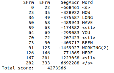
Since files with aligned transcripts included the timing in units corresponding to 10 ms, we were able to precisely extract features corresponding to single words from transcripts. All frames containing no words and described as 'silence', 'breathing', 'laughter' etc., were excluded from the data.

We excluded all the words that lasted more than 600 ms. This meant discarding some 2.6 % of spoken words and, since a typical speech speed is estimated to be 225 words per minute - meaning a mean duration of a word (excluding pauses) about 266 ms and a slow speech 100 words per minute - with one word lasting 600 ms, seemed to be a valid cut-off for getting rid of possibly misaligned words. Importantly, there was not a single word completely lost in the procedure - all of the rejected words had also 'shorter' realizations that were kept.
Similarly, we restricted the number of words in the sentence. Since the sentence length distribution had a long tail of outliers, we decided to keep sentences not longer than 25 words in order to decrease the computation time. This resulted in using 88 % of the data for the further analysis. For both words and sentences shorter than the threshold we used zero padding to keep the input size fixed.
While it is possible to use the sequence length as a parameter of the tf.nn.bidirectional_dynamic_rnn function used to initialize the network, it turned out that restricting the length of sequences was beneficial in terms of both computational efficiency and network's performance.
We used the gensim python library and precomputed embeddings (DOWNLOAD HERE). Words that were not the part of the model dictionary were assigned a zero embedding vector (precisely the length of embeddings is 300, so the zero embedding means a vector with 300 zeros).
Creating splits of data helps when it comes to training and evaluating the model. Instead of dividing in two parts, we created eight of them in order to be able to run 8-fold cross-validation of the model. This required taking into account a lot of different conditions under which the data was registered. Firstly, there were two scenarios - improvised and scripted conversations. Then, there were several couples of actors interacting with each other in several spatial arrangement. Since all of those factors could somehow bias the emotional rating, we made sure that each of those conditions is evenly represented in each split.
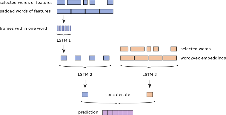
After the alignment words and audio features separate into two information streams in the model.

Audio features are processed in the hierarchical manner. LSTM 1 processes features of a single word. This is repeated for all of the words in the sentence. The output of this first layer is then passed as an input sequence to the LSTM 2. The second part of the model consists of a single LSTM 3 that is passed the sequence of word2vec embeddings. Outputs of these streams are then concatenated and regressed on the prediction vector. All the LSTM layers we used are bidirectional, meaning that they do the forward and backward pass of a sequence.
For the sake of comparing the performance of multi-modal architecture with learning on audio or texts only, the model can also be run in variants in which the streams are not concatenated and the output of LSTM 2 / LSTM 3 is regressed directly on the prediction vector.
Experiments conducted as a part of the project were a good lesson on training a recurrent network. One problem, that everyone is likely to face while working with LSTM nets, is the one of overfitting. This mean learning to perfectly represent the training data but failing to generalize (performing poorly on previously unseen data). Even with a small learning rate and dropout for the regularization of the network, it may be difficult to train if the data set is not big enough.
Then, training on text embeddings is definitely easier than training on audio files. Possibly this is caused by the complexity of the data - word2vec embedding for a given word is always the same, while the way the word is spoken differs between actors, but also between in time for a single person. Finally, in order to overcome this difficulties, one has to fine-tune a lot of hyper parameters and it's often not easy to choose them ad hoc. Running a parameter space exploration without knowing reasonable ranges for parameters is not a good idea especially when the training takes long.
One strategy that we applied was to start training on a smaller part of the data set in order to quickly see if the model can learn the problem and scale up - increase the data set with a small increase in the number of hidden cells. If that works one can try to play with learning rate, dropout, etc.
In our case, we used Adam optimizer, learning rates ranging from 5e-4 to 5e-6, dropout between consecutive layers with probabilities 0.3 - 0.5 and batch sizes around 20. We also used the exponential decay for the learning rate. Training for more epochs with a lower learning rate worked better than setting the learning rate higher at the beginning.
During the summer we developed and tested the multi-modal emotion prediction model and the data pipeline. While the training of the model is not yet finished and so the last goal of the project is not yet reached, the amount of challenges and little issues to take care of / read about along the way was definitely higher than anticipated while writing the proposal. The main issues we addressed are outlined above are just a fraction of ideas that we tried out. Let's just say the the learning curve of the humble programmer was way steeper than any of the curves registered by TensorBoard.
The project will continue after the GSoC period. Next steps are:
- finalizing the training
- comparing various architectures
- extending the data (another data sets)
'We' in this wiki page actually stands for 'my mentor - Karan Singla and I - Karolina Stosio'. Although I was the person doing the coding, it would not have happened without Karan, who did a tremendous job guiding me, motivating and providing ideas. BIG BIG THANKS TO YOU!
Another thank you goes to my fellow students from the WhatsApp GSoC channel who are a great and exciting crowd - good luck to all of you! Special thanks to Hammad and Ganesh, for staying in touch and motivating each other.
The last person that should be mentioned here is my boyfriend - thanks for all the coffee and support!
Finally, I'm extremely grateful for having a chance to participate in Google Summer of Code and I would definitely recommend it to any hesitant student. Go for it!