- W3, SQL Basics
- R4DS chapter 19
- SQLite Python, R
You can find examples and motivation in the resources.
In this lecture we will go through the basics of SQL. This includes the basic syntax for making queries to the database. This includes both retrieving and storing data in the database.
What is SQL? Structured Query Language (SQL) is a computer language that enables us to communicate and manipulate SQL databases(db) and it is one of the most widely used languages for db management.
There are many flavours (versions) of SQL. However, they all share the basic syntax as below and often only differ in the way the basic syntax is extended.
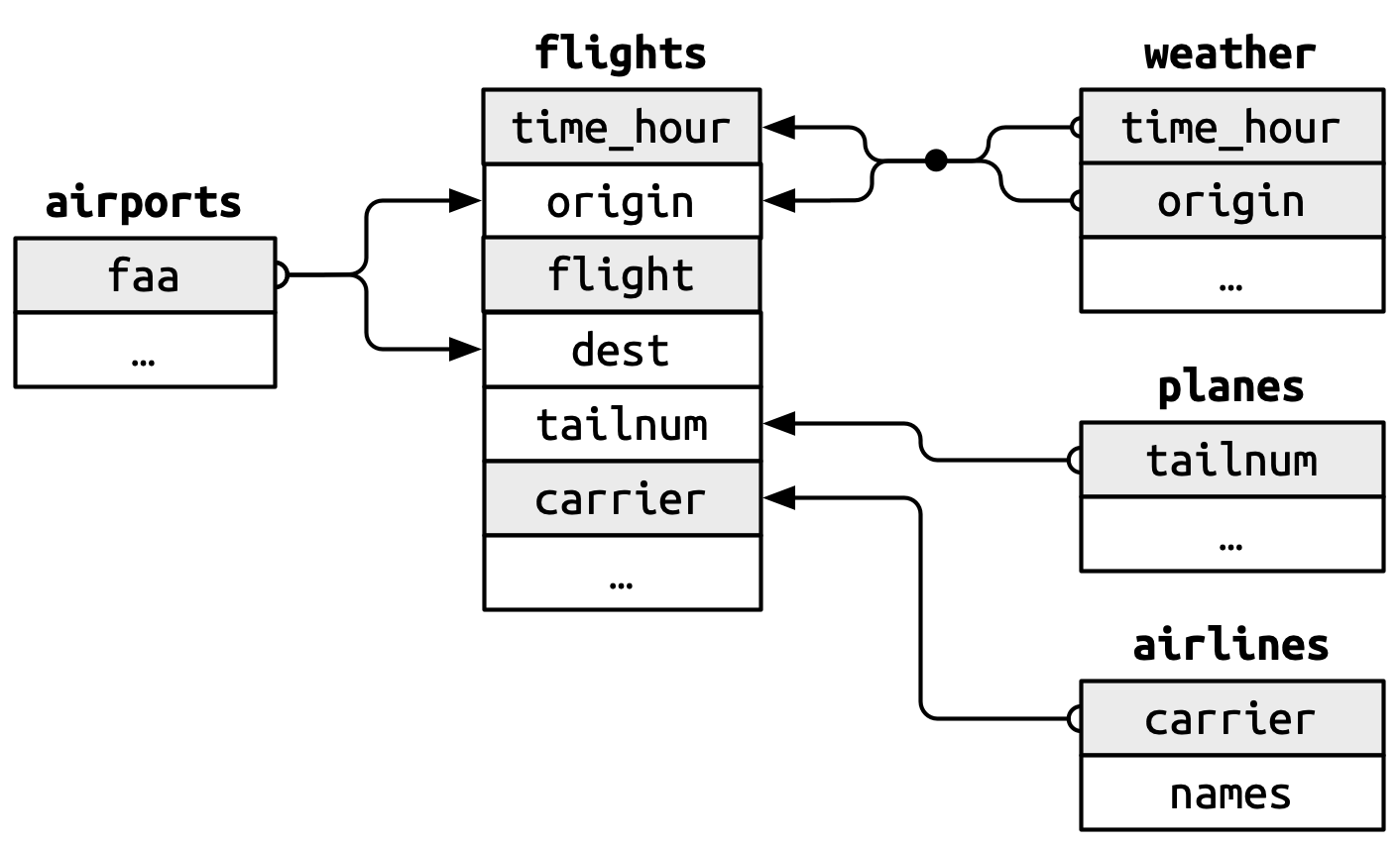
SQL is a Relational Database Management System (RDBMS), meaning that the data is stored in tables that are seperated based on the scope of the database. A nice illustration of how data is stored can be seen in the figure below.
Image borrowed from:https://r4ds.hadley.nz/
Here, the tables are seperated to reflect differring objects. We also see that the tables are linked or related to each other through specific variables (keys). This is where the name relational database comes from.
Writing an SQL query (a question or a requests) is similiar to speaking with the database. Once we get a grasp of the basic syntax we will be able to query the database for data in whatever form that is.
We use SELECT to determine the columns we want and FROM to specify the
table we want it from. Following the image above, we can make the following query.
SELECT carrier, dest, tailnum
FROM flights;
Make sure to end the query with ;
We can use SELELCT * to get all columns in the table. The query above is
the simplest query one can make in SQL.
We can add a layer of complexity by filtering the table. We can do this by
using the WHERE command. Continuing the example, we can make the following query.
SELECT carrier, dest, tailnum
FROM flights
WHERE dest='sweden';
Furthermore, we can use the logical operators AND, OR, NOT to perform logical chaining of conditions. The basic syntax is the following.
SELECT variable1, variable2, ... -- * if you want all variables
FROM table
WHERE condition1 AND/OR/NOT condition2 AND/OR/NOT condition3 ...;
To aggregate multiple tables into a single table we can use ... JOIN. The
syntax is similar to the previous lecture. ON specifies the key(s) to
join on. Continuing the example above the syntax is the following.
SELECT carrier, dest, tailnum, airlines.names
FROM flights
LEFT JOIN airlines ON flights.carrier = airlines.carrier;
Using the syntax described above, we can chain multiple operations to generate the desired table. You can see more operations on W3.
Since the SQL syntax has been adopted by both pandas and tidyverse, it will
not be difficult to learn the content above.
To start storing data, we need to create a table to store it in. We can do this
using the CREATE command. The query is as follows.
CREATE TABLE table_name (
  ...
);
To our table, we need to add columns (variable), we can do this by specifying the name of the column and datatype. We can also specify constraints on the variable. The query is as follows.
CREATE TABLE table_name (
  Variable1 datatype constraint,
  Variable2 datatype constraint,
  ...
);
Common constrains are NOT NULL, UNIQUE, PRIMARY KEY, FOREIGN KEY. There
are more constraints that can be added. They can be found on W3.
The unique identifier (id) of a row should be constrained with UNIQUE and it
must also be filled (NOT NULL). The PRIMARY KEY incorporates both constraints.
Therefore, it is good practice to specify the row id using the PRIMARY KEY
constraint.
An example of creating a table can look something like the following query.
CREATE TABLE Persons (
  name VARCHAR(255) NOT NULL,
  age INT,  -- It does not need to be specified
  id_number VARCHAR PRIMARY KEY
);
Specific datatypes can be looked up on W3.
To change a table that already exists we can use the ALTER command. Specific
ways to alter tables can be found on W3.
Putting it all together, the SQL query looks as follows.
CREATE TABLE Persons (
  Name VARCHAR(255) NOT NULL,
  Age INT,  -- It does not need to be specified
  ID_number VARCHAR(255) PRIMARY KEY
);

CREATE TABLE Computers (
  Computer_id INT PRIMARY KEY,
  Model VARCHAR(255),
  Brand VARCHAR(255),
  Owner VARCHAR(255) FOREIGN KEY REFERENCES Persons(ID_number)
)
Here, we create two tables and use FOREIGN KEY to link the owner of the
computer to a specific person using the id-number. If we later realise that we
want a person to have a variable specifying occupation, we can use the following
command.
ALTER TABLE Persons
ADD Occupation VARCHAR(255);
With a table created, we can add entries to the table. This can be done using
the INSERT command. The full syntax looks as follows.
INSERT INTO table_name (variable1, variable2, ...)
VALUES (value1, value2, ...)
Note that the order of the values should follow the order of the variables. Furthermore, if the constraints are violated we will get an error.
In the example above the query may look like
INSERT INTO Persons (Name, ID_number)
VALUES ('Taariq', '19000101-xxxx');
Since, the Age variable does not need to be filled in, the query will populate
the Persons table and have an empty cell (containing NULL) for the Age column.
We are only scratching the surface of SQL, there is a lot more to learn. However, with this basic knowledge we will be able to interact with databases. You can find more information in the listed resources (W3).
There are various libraries in Python and R to interact with SQL databases. We will primarily be working with SQLite databases since they are more accessible. Popular libraries are sqlite3 for Python and dbplyr for R.
