pyshqg is a python solver for the Marshal and Molteni (1993) quasi-geostrophic (QG) model.
QG models express the conservation of potential vorticity over time and are
meant to describe the large-scale circulation of the atmosphere under specific hypotheses.
This QG model is very special, because it is expressed in spherical harmonics and
because it encapsulates complex physical processes.
Install using pip:
$ pip install pyshqg
or using conda or mamba:
$ conda install conda-forge::pyshqg
More details can be found on this page.
Here is a sneak peak at how to use the package. First import all the machinery.
>>> import numpy as np
>>>
>>> from pyshqg.backend.numpy_backend import NumpyBackend as Backend
>>> from pyshqg.preprocessing.reference_data import load_test_data
>>> from pyshqg.core.constructors import construct_model, construct_integrator
Load the data and create the model and integrator.
>>> ds_test = load_test_data(internal_truncature=21, grid_truncature=31)
>>> backend = Backend(floatx='float64')
>>> model = construct_model(backend, ds_test.config)
>>> rk4 = construct_integrator(ds_test.config['rk4_integration'], model)
Perform one integration step and test against the test data.
>>> state = model.model_state(ds_test.spec_q.to_numpy())
>>> fwd_state = rk4.forward(state)
>>>
>>> def rms(x):
...     return np.sqrt(np.mean(np.square(x)))
>>>
>>> def rmse(x, y):
...     return rms(x-y)
>>>
>>> rms_ref = rms(ds_test.spec_rk4.to_numpy())
>>> rms_diff = rmse(
...     backend.to_numpy(fwd_state['spec_q']),
...     ds_test.spec_rk4.to_numpy(),
... )
>>> assert rms_diff < 1e-6 * rms_ref
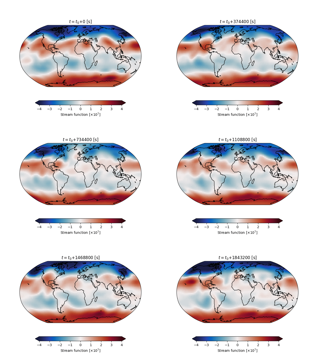
Run the model for a full trajectory and convert the output to an xarray.Dataset.
>>> state = model.model_state(ds_test.spec_q.to_numpy())
>>> trajectory = rk4.run(
...     state,
...     t_start=0,
...     num_snapshots=8,
...     num_steps_per_snapshot=10,
...     variables=('q', 'psi'),
... )
>>> trajectory.to_xarray()
<xarray.Dataset> Size: 14MB
Dimensions:  (time: 9, batch: 16, level: 3, lat: 32, lon: 64)
Coordinates:
  * time     (time) int64 72B 0 18000 36000 54000 ... 90000 108000 126000 144000
  * lat      (lat) float64 256B -85.76 -80.27 -74.74 ... 74.74 80.27 85.76
  * lon      (lon) float64 512B 180.0 185.6 191.2 196.9 ... 163.1 168.8 174.4
Dimensions without coordinates: batch, level
Data variables:
    q        (time, batch, level, lat, lon) float64 7MB -0.000298 ... -0.0001269
    psi      (time, batch, level, lat, lon) float64 7MB 1.445e+08 ... -1.38e+07
More details can be found on this page.
This python package is based on an original implementation of the model in Fortran written at LMD by XXX.
- make more example notebooks (see list below)
- fill in the documentation sections
- fill in docstrings, in particular with the convention used in the docs
- write pytorch/jax backends
- include unit tests in github CI
- apply linting and include it in github CI
Potential example notebooks:
- one notebook for each term of the QG model
- how to compute the forecast skill T15 vs T31 (as illustration)
- how to use tf backend to compute the grad
- gradient test for tf backend
- adjoint test for tf backend
- how to define a NN-based model error correction for the T21 and train it with dummy data

