Data Structure : Mathematical And Logical Model Of Organizing the interrelated data
-
A data structure is a way of organizing the data so that it can be used efficiently. Here, we have used the word efficiently, which in terms of both the space and time.
-
The data structure is not any programming language like C, C++, java, etc. It is a set of algorithms that we can use in any programming language to structure the data in the memory.
-
To structure the data in memory, 'n' number of algorithms were proposed, and all these algorithms are known as Abstract data types. These abstract data types are the set of rules.
There are two types of data structures:
Primitive data structure
Non-primitive data structure
The primitive data structures are primitive data types like:
intcharfloatdoublepointer
that can hold a single value.
The non-primitive data structure is divided into two types:
Linear data structure
Non-linear data structure
The arrangement of data in a sequential manner is known as a linear data structure. The data structures used for this purpose are:
ArraysLinked listStacksQueues
In these data structures, one element is connected to only one another element in a linear form.
When one element is connected to the 'n' number of elements known as a non-linear data structure. Like:
TreesGraphsHeapHash
In these case, the elements are arranged in a random manner.
Static data structure:It is a type of data structure where the size is allocated at the compile time. Therefore, the maximum size is fixed.Dynamic data structure:It is a type of data structure where the size is allocated at the run time. Therefore, the maximum size is flexibl
- A data structure is a way of organizing the data so that it can be used efficiently.
- Here, we have used the word efficiently, which in terms of both the space and time.
- For example, a stack is an ADT (Abstract data type) which uses either arrays or linked list data structure for the implementation.
- Therefore, we conclude that we require some data structure to implement a particular ADT.
An ADT tells what is to be done and data structure tells how it is to be done.In other words, we can say that ADT gives us the blueprint while data structure provides the implementation part.
The major or the common operations that can be performed on the data structures are:
Traversing:Visit all the lements in a data structure from one position to another.Searching:We can search for any element in a data structure.Sorting:We can sort the elements of a data structure either in an ascending or descending order.Insertion:We can also insert the new element in a data structure.Updation:We can also update the element, i.e., we can replace the element with another element.Deletion:We can also perform the delete operation to remove the element from the data structure.Merging:Combine two Data Structure of same type.
Efficiency:If the choice of a data structure for implementing a particular ADT is proper, it makes the program very efficient in terms of time and space.Reusability:The data structure provides reusability means that multiple client programs can use the data structure.Abstraction:The data structure specified by an ADT also provides the level of abstraction. The client cannot see the internal working of the data structure, so it does not have to worry about the implementation part. The client can only see the interface.
Basic Analysis Of Algorithm :
What Is Algorithm ?Time Complexity.Space Complexity.Rate Of Growth.Complexity Notation.Asymptotic Notation.Big OhThetaOmegs
Worst Case & Best Case.Pointers.Structure.
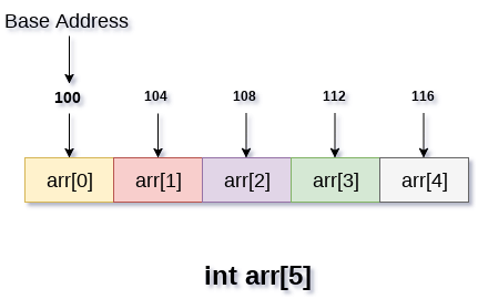
- Arrays are defined as the collection of similar type of data items stored at contiguous memory locations.
- Arrays are the derived data type in C programming language which can store the primitive type of data such as int, char, double, float, etc.
- Array is the simplest data structure where each data element can be randomly accessed by using its index number.
- In computer programming, the most of the cases requires to store the large number of data of similar type.
- To store such amount of data, we need to define a large number of variables.
- It would be very difficult to remember names of all the variables while writing the programs.
- Instead of naming all the variables with a different name, it is better to define an array and store all the elements into it.
To access any random element of an array we need the following information:
Base Address of the array.Size of an element in bytes.Relative Index :Number of elements present before the specified index of an element.
Byte address of element A[i]  = base address + size * Relative Index    ----------- 1
Relative Index : (i - first index)                                      ----------- i

Put i in 1 :
Byte address of element A[i]  = base address + size * (i - first index)
Traversing in Array means Visit all the elements of the array from Lower Bound Address to Upper Bound Address.
Implementation :
Step 01: Start
Step 02: [Initialize counter variable. ] Set i = LB.
Step 03: Repeat for i = LB to UB.
Step 04: Apply process to arr[i].
Step 05: [End of loop. ]
Step 06: Stop
| TIME COMPLEXITY | SPACE COMPLEXITY |
|---|---|
| Theta(n) | Theta(1) |
-
To Find the minimum Element in Array, we first assign the very first element as minimum
-
Then we can traverse through the whole array by comparing the assumed minimum element (Very first element in array).
-
If our minimum array element is greater then some element in array while traversing then we can assign that element as minimum element.
-
Like this we traverse till the end of the array and at the end the element present in minimum variable is the minimum element.
No Of Comparision Between The Elements : n-1
Implementation :
smallest = array[i] // first element
for i from 1 to length(array):
    element_i = array[i]
    if smallest > element_i
        smallest = element_i
smallest // this is our answer
| TIME COMPLEXITY | SPACE COMPLEXITY |
|---|---|
| Theta(n) | Theta(1) or O(1) |
-
To Find the Maximum Element in Array, we first assign the very first element as maximum
-
Then we can traverse through the whole array by comparing the assumed maximum element (Very first element in array).
-
If our maximum array element is smaller then some element in array while traversing then we can assign that element as maximum element.
-
Like this we traverse till the end of the array and at the end the element present in maximum variable is the maximum element.
No Of Comparision Between The Elements : n-1
Implementation :
Step 1: Start

Step 2: Declare array a[n] and variable i, large

Step 3: Read n from User and read all the elements of a[n]

Step 4: Initialize Variable i=1 and large=a[0]

Step 5: Repeat Until i<=n-1

           5.1 if(a[i]>large), set large=a[i]

           5.2 increment i=i+1

Step 6: Print "The largest element is": large

Step 7: Stop
| TIME COMPLEXITY | SPACE COMPLEXITY |
|---|---|
| Theta(n) | Theta(1) or O(1) |
   - No Of Comparision Between The Elements To find Minimum :              n-1
   - No Of Comparision Between The Elements To find Maximum :              n-1

   - Total Number Of Comparision To Find Min and Max        :              2n-2
2n-2 is The total number of comparision to find minimum and maximum : Complete Code :
- To reduce this comparision we can use one Method called :
- Divide the array into two parts and compare the maximums and minimums of the two parts to get the maximum and the minimum of the whole array.
Implementation (Algorithm) :
Pair MaxMin(array, array_size)
   if array_size = 1
      return element as both max and min
   else if arry_size = 2
      one comparison to determine max and min
      return that pair
   else    /* array_size  > 2 */
      recur for max and min of left half
      recur for max and min of right half
      one comparison determines true max of the two candidates
      one comparison determines true min of the two candidates
      return the pair of max and min
| TIME COMPLEXITY | SPACE COMPLEXITY |
|---|---|
| Theta(n) | Theta(n) |
   - No Of Comparision To make Two Lists of Max and Min :              n/2
   - No Of Comparision in Max list To find Maximum      :              n/2-1
   - No Of Comparision in Min list To find Minimum      :              n/2-1

   - Total Number Of Comparision To Find Min and Max    :              3n/2-2
Insert operation is to insert one or more data elements into an array. Based on the requirement, a new element can be added at the beginning, end, or any given index of array.
| TIME COMPLEXITY | SPACE COMPLEXITY | |
|---|---|---|
| Insertion At Beginning | O(n) | O(1) |
| Insertion At End | O(1) | O(1) |
| Insertion At Position | O(n) | O(1) |
Deletion refers to removing an existing element from the array and re-organizing all elements of an array.
| TIME COMPLEXITY | SPACE COMPLEXITY | |
|---|---|---|
| Deletion From Beginning | O(n) | O(1) |
| Deletion From End | O(1) | O(1) |
| Deletion From Position | O(n) | O(1) |
You can perform a search for an array element based on its value or its index.
| TIME COMPLEXITY | SPACE COMPLEXITY | |
|---|---|---|
| Linear Search | O(n) | O(1) |
| Binary Search | O(log n) | O(1) |
Combine two arrays in such a way that one array is appended to another array.
| TIME COMPLEXITY | SPACE COMPLEXITY | |
|---|---|---|
| Merging operation | O(m + n) | O(m + n) |
Update operation refers to updating an existing element from the array at a given index.
| TIME COMPLEXITY | SPACE COMPLEXITY | |
|---|---|---|
| Update operation | O(1) | O(1) |
- 2D array can be defined as an array of arrays.
- The 2D array is organized as matrices which can be represented as the collection of rows and columns.
int arr[max_rows][max_columns];
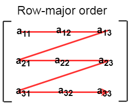
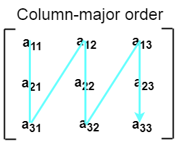
Mapping of 2D Array to 1D array is important because 2D arrays are the user's view but in memory or in computer's view they all are stored in 1D array either in Row Wise Order called Row Major Order OR Column Wise Order called Column Major Order.
- In row major ordering, all the rows of the 2D array are stored into the memory contiguously.
- First, the 1st row of the array is stored into the memory completely. - Then the 2nd row of the array is stored into the memory completely and so on till the last row.
- If array is declared by a[LBi...UBi][LBj...UBj] where,
LBi = Lower Bound of Row
LBj = Lower Bound of column
UBi = Upper Bound of row
UBj = Upper Bound of column
m = Number of rows (UBi - LBi + 1)
n = Number of column (UBj - LBj + 1)
- Then address of an element a[i][j] of the array stored in row major order is calculated as,
Address(a[i][j]) = Base_Address + size * [ (i-LBi)*n + (j-LBj) ]
- According to the column major ordering, all the columns of the 2D array are stored into the memory contiguously.
- First, the 1st column of the array is stored into the memory completely - Then the 2nd row of the array is stored into the memory completely and so on till the last column of the array.
- If array is declared by a[LBi...UBi][LBj...UBj] where,
LBi = Lower Bound of Row
LBj = Lower Bound of column
UBi = Upper Bound of row
UBj = Upper Bound of column
m = Number of rows (UBi - LBi + 1)
n = Number of column (UBj - LBj + 1)
- Then address of an element a[i][j] of the array stored in Column major order is calculated as,
Address(a[i][j]) = Base_Address + size * [ (j-LBj)*m + (i-LBi) ]
- Linked list is a linear data structure that includes a series of connected nodes.
- Linked list can be defined as the nodes that are randomly stored in the memory.
- A node in the linked list contains two parts, i.e., first is the data part and second is the address part.
- The last node of the list contains a pointer to the null.
- After array, linked list is the second most used data structure.
- In a linked list, every link contains a connection to another link.
limitations of arrays -
- The size of the array must be known in advance before using it in the program.
- Increasing the size of the array is a time taking process. It is almost impossible to expand the size of the array at run time.
- Inserting and deleting an element in the array needs shifting of all its predecessors.
Linked list is useful because -
- It allocates the memory dynamically.
- All the nodes of the linked list are non-contiguously stored in the memory and linked together with the help of pointers.
- In linked list, size is no longer a problem since we do not need to define its size at the time of declaration.
- List grows as per the program's demand and limited to the available memory space.
Memory usage -Each node of the linked list occupies two types of variables, i.e., one is a simple variable, and another one is the pointer variable.Traversal-If we have to access an element in the linked list, we cannot access it randomly, while in case of array we can randomly access it by index.Reverse traversing- Backtracking or reverse traversing is difficult in a linked list. In a doubly-linked list, it is easier but requires more memory to store the back pointer.
Insertion- This operation is performed to add an element into the list.Deletion- It is performed to delete an operation from the list.Traversing- It is performed to display the elements of the list.Search- It is performed to search an element from the list using the given key.
| TIME COMPLEXITY | SPACE COMPLEXITY | |
|---|---|---|
| Insertion At Beginning | O(1) | O(1) |
| Insertion At End | O(n) | O(1) |
| Insertion At Position | O(n) | O(1) |
| Insertion After Node | O(n) | O(1) |
| Insertion Before Node | O(n) | O(1) |
| TIME COMPLEXITY | SPACE COMPLEXITY | |
|---|---|---|
| Deletion From Beginning | O(1) | O(1) |
| Deletion From End | O(n) | O(1) |
| Deletion From Position | O(n) | O(1) |
- Doubly linked list is a complex type of linked list in which a node contains a pointer to the previous as well as the next node in the sequence.
- Therefore, in a doubly linked list, a node consists of three parts: node data, pointer to the next node in sequence (next pointer) , pointer to the previous node (previous pointer).
| TIME COMPLEXITY | SPACE COMPLEXITY | |
|---|---|---|
| Insertion At Beginning | O(1) | O(1) |
| Insertion At End | O(n) | O(1) |
| Insertion At Position | O(n) | O(1) |
| Insertion After Node | O(n) | O(1) |
| Insertion Before Node | O(n) | O(1) |
| TIME COMPLEXITY | SPACE COMPLEXITY | |
|---|---|---|
| Deletion From Beginning | O(1) | O(1) |
| Deletion From End | O(n) | O(1) |
| Deletion From Position | O(n) | O(1) |
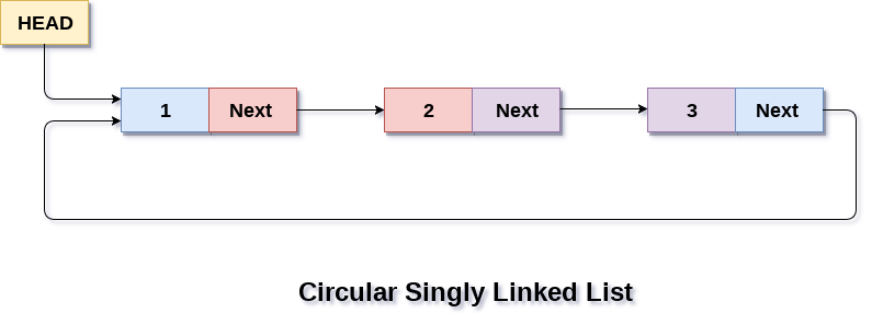
- In a circular Singly linked list, the last node of the list contains a pointer to the first node of the list.
- We can have circular singly linked list as well as circular doubly linked list.
- We traverse a circular singly linked list until we reach the same node where we started.
- The circular singly liked list has no beginning and no ending. There is no null value present in the next part of any of the nodes.
- Circular doubly linked list is a more complexed type of data structure in which a node contain pointers to its previous node as well as the next node.
- Circular doubly linked list doesn't contain NULL in any of the node. The last node of the list contains the address of the first node of the list.
- The first node of the list also contain address of the last node in its previous pointer.


