Welcome to Hold the Gold's D.C. housing analysis presentation#

The following analysis--by utilizing Zillow's extensive housing data--will examine the best real estate zip codes to invest in today.###

Goal:

To find the top 3 zipcodes for our savvy investors to deploy capital into for maximum financial return.

Assumptions:

You are an investor with a minimum of $100,000 to deploy upfront.
Your time horizon for investment is 5-10 years (this is not a liquid investment).
You seek to maximize growth potential by tapping into home value appreciation in one of America's fastest growing metro areas.
Your threshold for volatility is low (note that no investment is guaranteed and any investment with Hold the Gold is subject to future market conditions).

Background:

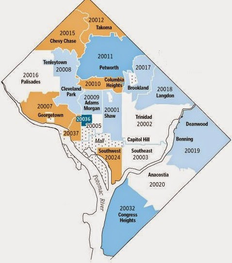
Why the D.C. metropolitan area?

max profit min volatitily max potential for home value increase while rental income supplmentation metro access upcoming fast growth trending area heavy insulation from federal govenrment home upcoming amazon headquarters future growth oritented risk vs profitability ROI yield

The DC area is home to numerous 10/10 GreatSchools Rated elementary, middle, and high schools 90-100 Most Competitive Redfin Compete Score Most homes get multiple offers, often with waived contingencies. Homes typically receive 1 offer. Homes sell for around list price and go pending in around 11 days. Hot Homes can sell for about 3% above list price and go pending in around 5 days.

walkscore.com Washington D.C. is the 7th most walkable large city in the US with 601,723 residents.

Washington D.C. has excellent public transportation and is somewhat bikeable.77 walk score 71 transit score

Exploratory Data Analysis:

## first import all relevant libraries
%matplotlib inline 
import pandas as pd
import numpy as np
import matplotlib.pyplot as plt
import datetime
import seaborn as sns
import statsmodels.api as sm
from statsmodels.tsa.stattools import adfuller
from statsmodels.tsa.seasonal import seasonal_decompose

## read in data
df=pd.read_csv("zillow_data.csv")

## preview data
df.head()

.dataframe tbody tr th {
    vertical-align: top;
}

.dataframe thead th {
    text-align: right;
}

</style>

	RegionID	RegionName	City	State	Metro	CountyName	SizeRank	1996-04	1996-05	1996-06	...	2017-07	2017-08	2017-09	2017-10	2017-11	2017-12	2018-01	2018-02	2018-03	2018-04
0	84654	60657	Chicago	IL	Chicago	Cook	1	334200.0	335400.0	336500.0	...	1005500	1007500	1007800	1009600	1013300	1018700	1024400	1030700	1033800	1030600
1	90668	75070	McKinney	TX	Dallas-Fort Worth	Collin	2	235700.0	236900.0	236700.0	...	308000	310000	312500	314100	315000	316600	318100	319600	321100	321800
2	91982	77494	Katy	TX	Houston	Harris	3	210400.0	212200.0	212200.0	...	321000	320600	320200	320400	320800	321200	321200	323000	326900	329900
3	84616	60614	Chicago	IL	Chicago	Cook	4	498100.0	500900.0	503100.0	...	1289800	1287700	1287400	1291500	1296600	1299000	1302700	1306400	1308500	1307000
4	93144	79936	El Paso	TX	El Paso	El Paso	5	77300.0	77300.0	77300.0	...	119100	119400	120000	120300	120300	120300	120300	120500	121000	121500

5 rows × 272 columns

## select only data from D.C. area
df_dc=df[df["State"]=="DC"]

## drop unneeded columns
## dropped RegionID, City, State, Metro, CountyName
df_dc=df_dc.drop(["RegionID", "City", "State", "Metro", "CountyName", "SizeRank"], axis=1)

##Rename RegionID to zipcode
df_dc.rename(columns={'RegionName': 'Zipcode'}, inplace=True)
df_dc.head()

.dataframe tbody tr th {
    vertical-align: top;
}

.dataframe thead th {
    text-align: right;
}

</style>

	Zipcode	1996-04	1996-05	1996-06	1996-07	1996-08	1996-09	1996-10	1996-11	1996-12	...	2017-07	2017-08	2017-09	2017-10	2017-11	2017-12	2018-01	2018-02	2018-03	2018-04
29	20002	94300.0	94000.0	93700.0	93600.0	93400.0	93400.0	93400.0	93600.0	94000.0	...	662800	668000	672200	673100	674600	678200	680900	683000	687500	691300
33	20009	178800.0	179200.0	179600.0	180000.0	180300.0	180700.0	181200.0	181800.0	182600.0	...	1020000	1027500	1034300	1040500	1047400	1055400	1065900	1076400	1081000	1078200
181	20011	118900.0	118500.0	118200.0	117800.0	117600.0	117400.0	117400.0	117500.0	117800.0	...	582200	586200	591200	593200	591200	589500	590800	599100	611400	619100
246	20019	91300.0	91000.0	90600.0	90400.0	90100.0	89900.0	89700.0	89600.0	89600.0	...	291100	296300	302500	306700	308800	310800	313400	314100	311800	308600
258	20001	92000.0	92600.0	93200.0	93900.0	94600.0	95400.0	96100.0	96800.0	97700.0	...	765000	768800	771200	773300	777600	780500	781600	785500	791400	793300

5 rows × 266 columns

## Reset dataframe index and drop old index related to original zillow dataset
df_dc.reset_index(drop=True)

.dataframe tbody tr th {
    vertical-align: top;
}

.dataframe thead th {
    text-align: right;
}

</style>

	Zipcode	1996-04	1996-05	1996-06	1996-07	1996-08	1996-09	1996-10	1996-11	1996-12	...	2017-07	2017-08	2017-09	2017-10	2017-11	2017-12	2018-01	2018-02	2018-03	2018-04
0	20002	94300.0	94000.0	93700.0	93600.0	93400.0	93400.0	93400.0	93600.0	94000.0	...	662800	668000	672200	673100	674600	678200	680900	683000	687500	691300
1	20009	178800.0	179200.0	179600.0	180000.0	180300.0	180700.0	181200.0	181800.0	182600.0	...	1020000	1027500	1034300	1040500	1047400	1055400	1065900	1076400	1081000	1078200
2	20011	118900.0	118500.0	118200.0	117800.0	117600.0	117400.0	117400.0	117500.0	117800.0	...	582200	586200	591200	593200	591200	589500	590800	599100	611400	619100
3	20019	91300.0	91000.0	90600.0	90400.0	90100.0	89900.0	89700.0	89600.0	89600.0	...	291100	296300	302500	306700	308800	310800	313400	314100	311800	308600
4	20001	92000.0	92600.0	93200.0	93900.0	94600.0	95400.0	96100.0	96800.0	97700.0	...	765000	768800	771200	773300	777600	780500	781600	785500	791400	793300
5	20020	104500.0	103800.0	103000.0	102200.0	101400.0	100600.0	100000.0	99500.0	99200.0	...	314700	317600	321800	324500	324800	324900	324900	327300	332800	337000
6	20008	450100.0	448200.0	446300.0	444500.0	442900.0	441600.0	440700.0	440100.0	440100.0	...	1501600	1508800	1509700	1506000	1509100	1514300	1519400	1527900	1539600	1545900
7	20003	130000.0	130100.0	130200.0	130400.0	130600.0	130900.0	131400.0	131900.0	132700.0	...	801000	807200	811900	813400	814600	814600	815300	817300	820200	820200
8	20032	85700.0	85500.0	85400.0	85200.0	85000.0	84800.0	84600.0	84400.0	84200.0	...	288100	293400	297800	301500	303700	304000	304600	306800	308200	307400
9	20016	362000.0	361200.0	360300.0	359400.0	358500.0	357700.0	357000.0	356500.0	356400.0	...	1202900	1198700	1196400	1190400	1184800	1183600	1186600	1190000	1196000	1199500
10	20010	110500.0	111200.0	112000.0	112900.0	113800.0	114900.0	116100.0	117400.0	118800.0	...	732800	741700	750900	756300	759300	761800	763500	767800	774700	778200
11	20007	358100.0	356000.0	353900.0	351700.0	349600.0	347500.0	345800.0	344400.0	343600.0	...	1329300	1330800	1324900	1314100	1303500	1296500	1293000	1291200	1291000	1290000
12	20024	209800.0	208200.0	206600.0	205000.0	203300.0	201900.0	200500.0	199300.0	198300.0	...	879200	866900	860100	864500	874100	878200	882300	885500	886900	885000
13	20017	121700.0	121400.0	121200.0	121000.0	120900.0	120900.0	121100.0	121400.0	121900.0	...	534300	534300	535300	535600	532600	531000	534400	542300	548400	548900
14	20018	123000.0	122400.0	121800.0	121200.0	120700.0	120400.0	120200.0	120200.0	120500.0	...	533200	535200	534700	533100	534500	538700	542200	548300	553800	554100
15	20037	277800.0	275800.0	273700.0	271600.0	269500.0	267600.0	265800.0	264200.0	263100.0	...	906400	914900	918700	923400	938900	953100	967600	990100	1013500	1019600
16	20015	312400.0	311000.0	309800.0	308700.0	307900.0	307400.0	307300.0	307700.0	308800.0	...	1000500	1004000	1005300	1003700	1002900	1003600	1004400	1006400	1007200	1004000
17	20012	185000.0	184900.0	184700.0	184400.0	184100.0	183900.0	183700.0	183800.0	184200.0	...	688500	692000	696100	699400	703800	709400	714400	720100	727400	730700

18 rows × 266 columns

##cast all zipcodes to string from integer
df_dc["Zipcode"]=df_dc["Zipcode"].astype(str)

## transpose dates to rows
df_dc=df_dc.transpose()
df_dc.head()

.dataframe tbody tr th {
    vertical-align: top;
}

.dataframe thead th {
    text-align: right;
}

</style>

	29	33	181	246	258	402	1263	1448	1707	2066	2581	2653	5297	5339	5453	5805	6484	6887
Zipcode	20002	20009	20011	20019	20001	20020	20008	20003	20032	20016	20010	20007	20024	20017	20018	20037	20015	20012
1996-04	94300	178800	118900	91300	92000	104500	450100	130000	85700	362000	110500	358100	209800	121700	123000	277800	312400	185000
1996-05	94000	179200	118500	91000	92600	103800	448200	130100	85500	361200	111200	356000	208200	121400	122400	275800	311000	184900
1996-06	93700	179600	118200	90600	93200	103000	446300	130200	85400	360300	112000	353900	206600	121200	121800	273700	309800	184700
1996-07	93600	180000	117800	90400	93900	102200	444500	130400	85200	359400	112900	351700	205000	121000	121200	271600	308700	184400

## Renaming all columns to reflect the 18 zipcodes of D.C.

new_header=df_dc.iloc[0] ##grab all first row data for the column headers
df_dc=df_dc[1:] ## take all rows after first row
df_dc.columns=new_header ## assign all column headers to be equal to row 0 data

df_dc.head()

.dataframe tbody tr th {
    vertical-align: top;
}

.dataframe thead th {
    text-align: right;
}

</style>

Zipcode	20002	20009	20011	20019	20001	20020	20008	20003	20032	20016	20010	20007	20024	20017	20018	20037	20015	20012
1996-04	94300	178800	118900	91300	92000	104500	450100	130000	85700	362000	110500	358100	209800	121700	123000	277800	312400	185000
1996-05	94000	179200	118500	91000	92600	103800	448200	130100	85500	361200	111200	356000	208200	121400	122400	275800	311000	184900
1996-06	93700	179600	118200	90600	93200	103000	446300	130200	85400	360300	112000	353900	206600	121200	121800	273700	309800	184700
1996-07	93600	180000	117800	90400	93900	102200	444500	130400	85200	359400	112900	351700	205000	121000	121200	271600	308700	184400
1996-08	93400	180300	117600	90100	94600	101400	442900	130600	85000	358500	113800	349600	203300	120900	120700	269500	307900	184100

df_dc.index=pd.to_datetime(df_dc.index)
df_dc.info()

<class 'pandas.core.frame.DataFrame'>
DatetimeIndex: 265 entries, 1996-04-01 to 2018-04-01
Data columns (total 18 columns):
20002    265 non-null object
20009    265 non-null object
20011    265 non-null object
20019    265 non-null object
20001    265 non-null object
20020    265 non-null object
20008    265 non-null object
20003    265 non-null object
20032    265 non-null object
20016    265 non-null object
20010    265 non-null object
20007    265 non-null object
20024    265 non-null object
20017    265 non-null object
20018    265 non-null object
20037    265 non-null object
20015    265 non-null object
20012    265 non-null object
dtypes: object(18)
memory usage: 39.3+ KB

df_dc.reset_index()
df_dc.head()

.dataframe tbody tr th {
    vertical-align: top;
}

.dataframe thead th {
    text-align: right;
}

</style>

Zipcode	20002	20009	20011	20019	20001	20020	20008	20003	20032	20016	20010	20007	20024	20017	20018	20037	20015	20012
1996-04-01	94300	178800	118900	91300	92000	104500	450100	130000	85700	362000	110500	358100	209800	121700	123000	277800	312400	185000
1996-05-01	94000	179200	118500	91000	92600	103800	448200	130100	85500	361200	111200	356000	208200	121400	122400	275800	311000	184900
1996-06-01	93700	179600	118200	90600	93200	103000	446300	130200	85400	360300	112000	353900	206600	121200	121800	273700	309800	184700
1996-07-01	93600	180000	117800	90400	93900	102200	444500	130400	85200	359400	112900	351700	205000	121000	121200	271600	308700	184400
1996-08-01	93400	180300	117600	90100	94600	101400	442900	130600	85000	358500	113800	349600	203300	120900	120700	269500	307900	184100

## cast all prices from strings to integers
df_dc=df_dc.astype(int)

Plotting Zipcode Trends:

df_dc.plot(figsize=(17,8))
plt.title("Housing Price Trends ")
plt.xlabel('Year')
plt.ylabel('Home Price $')
##top 3 zip codes have consistently been top 3 performers for the last 20 years
## bottom 3 zipcodes display little change over time in price compared to top priced zip codes
## all zip codes display a similar trend with a an inflection point for the year 2008 (housing recession)

Text(0, 0.5, 'Home Price $')

Testing for Stationarity:

#function to plot rolling mean and SD:
def test_stationarity(timeseries, window):
    
    #Defining rolling statistics
    rolmean = timeseries.rolling(window=window).mean()
    rolstd = timeseries.rolling(window=window).std()

    #Plot rolling statistics:
    fig = plt.figure(figsize=(12, 8))
    orig = plt.plot(timeseries.iloc[window:], color='blue',label='Original')
    mean = plt.plot(rolmean, color='red', label='Rolling Mean')
    std = plt.plot(rolstd, color='black', label = 'Rolling Std')
    plt.legend(loc='upper left')
    plt.title('Rolling Mean & Standard Deviation')
    plt.show()

#call function to test the stationarity of the untransformed dataset; window = 22 years (full time range available)
test_stationarity(df_dc, 12)

##the assumption of stationarity is not met, as rolling mean is not constant over time

df_dc.plot(figsize = (20,15), subplots=True, legend=True)
plt.show()

df_dc.plot(figsize = (20,6), style = ".b")
import matplotlib.pyplot as plt
plt.show()

def dickey_fuller_test_ind_zip(zip_code):
    dftest = adfuller(zip_code)

    # Extract and display test results in a user friendly manner
    dfoutput = pd.Series(dftest[0:4], index=['Test Statistic','p-value','#Lags Used','Number of Observations Used'])
    for key,value in dftest[4].items():
        dfoutput['Critical Value (%s)'%key] = value
    print(dftest)

    print ('Results of Dickey-Fuller Test:')

    print(dfoutput)

def dickey_fuller_test_all_zip(df_dc):
    for col in df_dc.columns:
        dftest = adfuller(df_dc[col])
        dfoutput = pd.Series(dftest[0:4], index=['Test Statistic','p-value','#Lags Used','Number of Observations Used'])
#         for key,value in dftest[4].items():
#             dfoutput['Critical Value (%s)'%key] = value
        print(dftest)

        print ('Results of Dickey-Fuller Test:')
        print ('\n')
        print(dfoutput)

dickey_fuller_test_all_zip(df_dc)

(-0.5461367553749569, 0.8826944742052973, 15, 249, {'1%': -3.4568881317725864, '5%': -2.8732185133016057, '10%': -2.5729936189738876}, 3920.545252411292)
Results of Dickey-Fuller Test:


Test Statistic                  -0.546137
p-value                          0.882694
#Lags Used                      15.000000
Number of Observations Used    249.000000
dtype: float64
(-1.1189148131844875, 0.7074702578291568, 14, 250, {'1%': -3.456780859712, '5%': -2.8731715065600003, '10%': -2.572968544}, 4121.4250877836475)
Results of Dickey-Fuller Test:


Test Statistic                  -1.118915
p-value                          0.707470
#Lags Used                      14.000000
Number of Observations Used    250.000000
dtype: float64
(-0.6378014655638256, 0.8622096679826863, 16, 248, {'1%': -3.4569962781990573, '5%': -2.8732659015936024, '10%': -2.573018897632674}, 3985.499935374562)
Results of Dickey-Fuller Test:


Test Statistic                  -0.637801
p-value                          0.862210
#Lags Used                      16.000000
Number of Observations Used    248.000000
dtype: float64
(-1.783928143277446, 0.38846961035679833, 14, 250, {'1%': -3.456780859712, '5%': -2.8731715065600003, '10%': -2.572968544}, 3707.12143693434)
Results of Dickey-Fuller Test:


Test Statistic                  -1.783928
p-value                          0.388470
#Lags Used                      14.000000
Number of Observations Used    250.000000
dtype: float64
(-0.7863232950406892, 0.8231065220249374, 13, 251, {'1%': -3.4566744514553016, '5%': -2.8731248767783426, '10%': -2.5729436702592023}, 4087.3255592934966)
Results of Dickey-Fuller Test:


Test Statistic                  -0.786323
p-value                          0.823107
#Lags Used                      13.000000
Number of Observations Used    251.000000
dtype: float64
(-0.8510469518706897, 0.8036658555525436, 11, 253, {'1%': -3.4564641849494113, '5%': -2.873032730098417, '10%': -2.572894516864816}, 3886.6717815895763)
Results of Dickey-Fuller Test:


Test Statistic                  -0.851047
p-value                          0.803666
#Lags Used                      11.000000
Number of Observations Used    253.000000
dtype: float64
(-2.1246519573586, 0.23471814510978506, 15, 249, {'1%': -3.4568881317725864, '5%': -2.8732185133016057, '10%': -2.5729936189738876}, 4604.50885324107)
Results of Dickey-Fuller Test:


Test Statistic                  -2.124652
p-value                          0.234718
#Lags Used                      15.000000
Number of Observations Used    249.000000
dtype: float64
(-1.351554093376601, 0.6052689614445382, 14, 250, {'1%': -3.456780859712, '5%': -2.8731715065600003, '10%': -2.572968544}, 4015.436515742065)
Results of Dickey-Fuller Test:


Test Statistic                  -1.351554
p-value                          0.605269
#Lags Used                      14.000000
Number of Observations Used    250.000000
dtype: float64
(-1.6606726131817435, 0.4514804598856628, 15, 249, {'1%': -3.4568881317725864, '5%': -2.8732185133016057, '10%': -2.5729936189738876}, 3854.570300542063)
Results of Dickey-Fuller Test:


Test Statistic                  -1.660673
p-value                          0.451480
#Lags Used                      15.000000
Number of Observations Used    249.000000
dtype: float64
(-1.893209383580719, 0.33526234346022366, 16, 248, {'1%': -3.4569962781990573, '5%': -2.8732659015936024, '10%': -2.573018897632674}, 4162.106286545486)
Results of Dickey-Fuller Test:


Test Statistic                  -1.893209
p-value                          0.335262
#Lags Used                      16.000000
Number of Observations Used    248.000000
dtype: float64
(-0.7829695413213618, 0.8240735226075573, 15, 249, {'1%': -3.4568881317725864, '5%': -2.8732185133016057, '10%': -2.5729936189738876}, 4062.1446310261886)
Results of Dickey-Fuller Test:


Test Statistic                  -0.782970
p-value                          0.824074
#Lags Used                      15.000000
Number of Observations Used    249.000000
dtype: float64
(-2.5638865628678444, 0.10069322265750907, 15, 249, {'1%': -3.4568881317725864, '5%': -2.8732185133016057, '10%': -2.5729936189738876}, 4290.592655898537)
Results of Dickey-Fuller Test:


Test Statistic                  -2.563887
p-value                          0.100693
#Lags Used                      15.000000
Number of Observations Used    249.000000
dtype: float64
(-1.1207233032741089, 0.7067373400486667, 15, 249, {'1%': -3.4568881317725864, '5%': -2.8732185133016057, '10%': -2.5729936189738876}, 4431.973326532635)
Results of Dickey-Fuller Test:


Test Statistic                  -1.120723
p-value                          0.706737
#Lags Used                      15.000000
Number of Observations Used    249.000000
dtype: float64
(-1.0270059246675498, 0.7432875350502444, 14, 250, {'1%': -3.456780859712, '5%': -2.8731715065600003, '10%': -2.572968544}, 3918.9590569410925)
Results of Dickey-Fuller Test:


Test Statistic                  -1.027006
p-value                          0.743288
#Lags Used                      14.000000
Number of Observations Used    250.000000
dtype: float64
(-1.367309827474695, 0.5978440314731485, 14, 250, {'1%': -3.456780859712, '5%': -2.8731715065600003, '10%': -2.572968544}, 3957.9708796315267)
Results of Dickey-Fuller Test:


Test Statistic                  -1.367310
p-value                          0.597844
#Lags Used                      14.000000
Number of Observations Used    250.000000
dtype: float64
(-1.5877703821992597, 0.48973390196328087, 15, 249, {'1%': -3.4568881317725864, '5%': -2.8732185133016057, '10%': -2.5729936189738876}, 4475.32772592358)
Results of Dickey-Fuller Test:


Test Statistic                  -1.587770
p-value                          0.489734
#Lags Used                      15.000000
Number of Observations Used    249.000000
dtype: float64
(-2.3368984183338486, 0.16034343125044997, 13, 251, {'1%': -3.4566744514553016, '5%': -2.8731248767783426, '10%': -2.5729436702592023}, 4072.020968218638)
Results of Dickey-Fuller Test:


Test Statistic                  -2.336898
p-value                          0.160343
#Lags Used                      13.000000
Number of Observations Used    251.000000
dtype: float64
(-1.2407229603830006, 0.6558371166009613, 15, 249, {'1%': -3.4568881317725864, '5%': -2.8732185133016057, '10%': -2.5729936189738876}, 4055.559672390052)
Results of Dickey-Fuller Test:


Test Statistic                  -1.240723
p-value                          0.655837
#Lags Used                      15.000000
Number of Observations Used    249.000000
dtype: float64

Detrending data:

Group 1 Zip Codes: High Performance: 20008, 20007, 20016

Zip code 20008

dickey_fuller_test_ind_zip(df_dc['20008'])

(-2.1246519573586, 0.23471814510978506, 15, 249, {'1%': -3.4568881317725864, '5%': -2.8732185133016057, '10%': -2.5729936189738876}, 4604.50885324107)
Results of Dickey-Fuller Test:
Test Statistic                  -2.124652
p-value                          0.234718
#Lags Used                      15.000000
Number of Observations Used    249.000000
Critical Value (1%)             -3.456888
Critical Value (5%)             -2.873219
Critical Value (10%)            -2.572994
dtype: float64

test_stationarity(df_dc['20008'], 12)

## Log transformation on zipcode 20008 and then perfomed Dickey_fuller test
##after transformation, p-value within critical range and can reject null hypothesis (stationry assumption met)

#log transformation and dickey-fuller test for 20008 zip code
log_20008 = pd.Series(np.log(df_dc["20008"]))
dickey_fuller_test_ind_zip(log_20008)

(-3.44412382463593, 0.00954356745494694, 15, 249, {'1%': -3.4568881317725864, '5%': -2.8732185133016057, '10%': -2.5729936189738876}, -2366.5978750425043)
Results of Dickey-Fuller Test:
Test Statistic                  -3.444124
p-value                          0.009544
#Lags Used                      15.000000
Number of Observations Used    249.000000
Critical Value (1%)             -3.456888
Critical Value (5%)             -2.873219
Critical Value (10%)            -2.572994
dtype: float64

#plot log transformation for 20008 zip code
fig = plt.figure(figsize=(12,6))
plt.plot(log_20008, color="blue")
plt.xlabel("month", fontsize=14)
plt.ylabel("log(monthly sales)", fontsize=14)
plt.show()

test_stationarity(log_20008, 12)

dickey_fuller_test_ind_zip(log_20008)

(-3.44412382463593, 0.00954356745494694, 15, 249, {'1%': -3.4568881317725864, '5%': -2.8732185133016057, '10%': -2.5729936189738876}, -2366.5978750425043)
Results of Dickey-Fuller Test:
Test Statistic                  -3.444124
p-value                          0.009544
#Lags Used                      15.000000
Number of Observations Used    249.000000
Critical Value (1%)             -3.456888
Critical Value (5%)             -2.873219
Critical Value (10%)            -2.572994
dtype: float64

Group 2: High Medium Performing Zip codes: 20024, 20009, 20015, 20018, 20037

Zip code 20024:

test_stationarity(df_dc['20024'],12)

dickey_fuller_test_ind_zip(df_dc['20024'])

(-1.1207233032741089, 0.7067373400486667, 15, 249, {'1%': -3.4568881317725864, '5%': -2.8732185133016057, '10%': -2.5729936189738876}, 4431.973326532635)
Results of Dickey-Fuller Test:
Test Statistic                  -1.120723
p-value                          0.706737
#Lags Used                      15.000000
Number of Observations Used    249.000000
Critical Value (1%)             -3.456888
Critical Value (5%)             -2.873219
Critical Value (10%)            -2.572994
dtype: float64

transform_20024= np.log(df_dc['20024']).diff().diff()

transform_20024.dropna(inplace=True)

transform_20024.head()

1996-06-01   -0.000059
1996-07-01   -0.000060
1996-08-01   -0.000553
1996-09-01    0.001417
1996-10-01   -0.000048
Name: 20024, dtype: float64

test_stationarity(transform_20024, 12)

dickey_fuller_test_ind_zip(transform_20024)

(-7.56980371999187, 2.8612220487957537e-11, 13, 249, {'1%': -3.4568881317725864, '5%': -2.8732185133016057, '10%': -2.5729936189738876}, -2203.9452901254763)
Results of Dickey-Fuller Test:
Test Statistic                -7.569804e+00
p-value                        2.861222e-11
#Lags Used                     1.300000e+01
Number of Observations Used    2.490000e+02
Critical Value (1%)           -3.456888e+00
Critical Value (5%)           -2.873219e+00
Critical Value (10%)          -2.572994e+00
dtype: float64

Group 3: Low Middle Performers: 20002, 20010, 20001, 20003, 200017,20012, 20011

Zip code 20002

dickey_fuller_test_ind_zip(df_dc['20002'])

(-0.5461367553749569, 0.8826944742052973, 15, 249, {'1%': -3.4568881317725864, '5%': -2.8732185133016057, '10%': -2.5729936189738876}, 3920.545252411292)
Results of Dickey-Fuller Test:
Test Statistic                  -0.546137
p-value                          0.882694
#Lags Used                      15.000000
Number of Observations Used    249.000000
Critical Value (1%)             -3.456888
Critical Value (5%)             -2.873219
Critical Value (10%)            -2.572994
dtype: float64

test_stationarity(df_dc['20002'], 12)

transform_20002= np.log(df_dc['20002']).diff().diff()

transform_20002.dropna(inplace=True)

test_stationarity(transform_20002, 12)

dickey_fuller_test_ind_zip(transform_20002)

(-4.075268710551853, 0.0010638155911648214, 12, 250, {'1%': -3.456780859712, '5%': -2.8731715065600003, '10%': -2.572968544}, -2459.84049471383)
Results of Dickey-Fuller Test:
Test Statistic                  -4.075269
p-value                          0.001064
#Lags Used                      12.000000
Number of Observations Used    250.000000
Critical Value (1%)             -3.456781
Critical Value (5%)             -2.873172
Critical Value (10%)            -2.572969
dtype: float64

Low Performers: 20032, 20020, 20019

Zip code 20032:

dickey_fuller_test_ind_zip(df_dc['20032'])

(-1.6606726131817435, 0.4514804598856628, 15, 249, {'1%': -3.4568881317725864, '5%': -2.8732185133016057, '10%': -2.5729936189738876}, 3854.570300542063)
Results of Dickey-Fuller Test:
Test Statistic                  -1.660673
p-value                          0.451480
#Lags Used                      15.000000
Number of Observations Used    249.000000
Critical Value (1%)             -3.456888
Critical Value (5%)             -2.873219
Critical Value (10%)            -2.572994
dtype: float64

test_stationarity(df_dc['20032'], 12)

transform_20032= np.log(df_dc['20032']).diff().diff()

transform_20032.dropna(inplace=True)

transform_20032.head()

1996-06-01    0.001166
1996-07-01   -0.001174
1996-08-01   -0.000006
1996-09-01   -0.000006
1996-10-01   -0.000006
Name: 20032, dtype: float64

test_stationarity(transform_20032,12)

dickey_fuller_test_ind_zip(transform_20032)

(-5.676570169441492, 8.67738969521844e-07, 13, 249, {'1%': -3.4568881317725864, '5%': -2.8732185133016057, '10%': -2.5729936189738876}, -2179.5784751300043)
Results of Dickey-Fuller Test:
Test Statistic                -5.676570e+00
p-value                        8.677390e-07
#Lags Used                     1.300000e+01
Number of Observations Used    2.490000e+02
Critical Value (1%)           -3.456888e+00
Critical Value (5%)           -2.873219e+00
Critical Value (10%)          -2.572994e+00
dtype: float64

Creating Final Dataset for Modeling

df_dc_final4=df_dc.copy()

df_dc_final4.head()

.dataframe tbody tr th {
    vertical-align: top;
}

.dataframe thead th {
    text-align: right;
}

</style>

Zipcode	20002	20009	20011	20019	20001	20020	20008	20003	20032	20016	20010	20007	20024	20017	20018	20037	20015	20012
1996-04-01	94300	178800	118900	91300	92000	104500	450100	130000	85700	362000	110500	358100	209800	121700	123000	277800	312400	185000
1996-05-01	94000	179200	118500	91000	92600	103800	448200	130100	85500	361200	111200	356000	208200	121400	122400	275800	311000	184900
1996-06-01	93700	179600	118200	90600	93200	103000	446300	130200	85400	360300	112000	353900	206600	121200	121800	273700	309800	184700
1996-07-01	93600	180000	117800	90400	93900	102200	444500	130400	85200	359400	112900	351700	205000	121000	121200	271600	308700	184400
1996-08-01	93400	180300	117600	90100	94600	101400	442900	130600	85000	358500	113800	349600	203300	120900	120700	269500	307900	184100

df_dc_final4=df_dc_final4[['20008','20024','20002','20032']]
df_dc_final4.head()

.dataframe tbody tr th {
    vertical-align: top;
}

.dataframe thead th {
    text-align: right;
}

</style>

Zipcode	20008	20024	20002	20032
1996-04-01	450100	209800	94300	85700
1996-05-01	448200	208200	94000	85500
1996-06-01	446300	206600	93700	85400
1996-07-01	444500	205000	93600	85200
1996-08-01	442900	203300	93400	85000

df_dc_final4['20008']=log_20008
df_dc_final4['20024']=transform_20024
df_dc_final4['20002']=transform_20002
df_dc_final4['20032']=transform_20032

df_dc_final4.dropna(inplace=True)
df_dc_final4.info()

<class 'pandas.core.frame.DataFrame'>
DatetimeIndex: 263 entries, 1996-06-01 to 2018-04-01
Data columns (total 4 columns):
20008    263 non-null float64
20024    263 non-null float64
20002    263 non-null float64
20032    263 non-null float64
dtypes: float64(4)
memory usage: 10.3 KB

df_dc_final4.to_csv("df_dc_final4.csv")

ARIMA:

!pip install pmdarima

Requirement already satisfied: pmdarima in /anaconda3/lib/python3.7/site-packages (1.2.1)
Requirement already satisfied: joblib>=0.11 in /anaconda3/lib/python3.7/site-packages (from pmdarima) (0.13.2)
Requirement already satisfied: pandas>=0.19 in /anaconda3/lib/python3.7/site-packages (from pmdarima) (0.23.4)
Requirement already satisfied: six>=1.5 in /anaconda3/lib/python3.7/site-packages (from pmdarima) (1.12.0)
Requirement already satisfied: scipy<1.3,>=1.2 in /anaconda3/lib/python3.7/site-packages (from pmdarima) (1.2.2)
Requirement already satisfied: Cython>=0.29 in /anaconda3/lib/python3.7/site-packages (from pmdarima) (0.29.2)
Requirement already satisfied: statsmodels>=0.9.0 in /anaconda3/lib/python3.7/site-packages (from pmdarima) (0.9.0)
Requirement already satisfied: scikit-learn>=0.19 in /anaconda3/lib/python3.7/site-packages (from pmdarima) (0.20.1)
Requirement already satisfied: numpy>=1.15 in /anaconda3/lib/python3.7/site-packages (from pmdarima) (1.15.4)
Requirement already satisfied: python-dateutil>=2.5.0 in /anaconda3/lib/python3.7/site-packages (from pandas>=0.19->pmdarima) (2.7.5)
Requirement already satisfied: pytz>=2011k in /anaconda3/lib/python3.7/site-packages (from pandas>=0.19->pmdarima) (2018.7)

# Load specific forecasting tools
from statsmodels.tsa.arima_model import ARMA,ARMAResults,ARIMA,ARIMAResults
from statsmodels.graphics.tsaplots import plot_acf,plot_pacf # for determining (p,q) orders
from statsmodels.tsa.stattools import adfuller
from statsmodels.graphics.tsaplots import plot_acf,plot_pacf
import statsmodels.api as sm
from statsmodels.tsa.statespace.sarimax import SARIMAX
from statsmodels.graphics.tsaplots import plot_acf,plot_pacf # for determining (p,q) orders
from statsmodels.tsa.seasonal import seasonal_decompose      # for ETS Plots

from pmdarima import auto_arima                              # for determining ARIMA orders
# Ignore harmless warnings
import warnings
warnings.filterwarnings("ignore")

---------------------------------------------------------------------------

AttributeError                            Traceback (most recent call last)

<ipython-input-96-fd588773a7f5> in <module>
      9 from statsmodels.tsa.seasonal import seasonal_decompose      # for ETS Plots
     10 
---> 11 from pmdarima import auto_arima                              # for determining ARIMA orders
     12 # Ignore harmless warnings
     13 import warnings


/anaconda3/lib/python3.7/site-packages/pmdarima/__init__.py in <module>
     27 
     28     # Stuff we want at top-level
---> 29     from .arima import auto_arima, ARIMA, AutoARIMA
     30     from .utils import acf, autocorr_plot, c, pacf, plot_acf, plot_pacf
     31 


/anaconda3/lib/python3.7/site-packages/pmdarima/arima/__init__.py in <module>
      3 # Author: Taylor Smith <[email protected]>
      4 
----> 5 from .approx import *
      6 from .arima import *
      7 from .auto import *


/anaconda3/lib/python3.7/site-packages/pmdarima/arima/approx.py in <module>
     17 # and since the platform might name the .so file something funky (like
     18 # _arima.cpython-35m-darwin.so), import this absolutely and not relatively.
---> 19 from pmdarima.arima._arima import C_Approx
     20 
     21 __all__ = [


/anaconda3/lib/python3.7/site-packages/pmdarima/arima/_arima.cpython-37m-darwin.so in init pmdarima.arima._arima()


AttributeError: type object 'pmdarima.arima._arima.array' has no attribute '__reduce_cython__'

title = 'Autocorrelation: Washington DC 20008 Zipcode'
lags = 40
plot_acf(df_dc['20008'],title=title,lags=lags);

title = 'Partial Autocorrelation: Washington DC 20008 Zipcode'
lags = 40
plot_pacf(df_dc['20008'],title=title,lags=lags);

import warnings
import itertools
import pandas as pd
import numpy as np
import matplotlib.pyplot as plt
import statsmodels.api as sm

train_data = df_dc_final4['1966-01-04':'2013-01-04']
test_data= df_dc_final4['2013-01-05':'2018-04-01']

ARIMA Zip: 20008

auto_arima(df_dc_final4['20008'],seasonal=True).summary()

---------------------------------------------------------------------------

NameError                                 Traceback (most recent call last)

<ipython-input-101-5cfffea136f2> in <module>
----> 1 auto_arima(df_dc_final4['20008'],seasonal=True).summary()


NameError: name 'auto_arima' is not defined

stepwise_fit = auto_arima(df_dc_final4['20008'], start_p=0, start_q=0,
                         max_p=2, max_q=2, m=12,
                         seasonal=True,
                         d=None, trace=True,
                         error_action='ignore',   # we don't want to know if an order does not work
                         suppress_warnings=True,  # we don't want convergence warnings
                         stepwise=True)           # set to stepwise

stepwise_fit.summary()

---------------------------------------------------------------------------

NameError                                 Traceback (most recent call last)

<ipython-input-102-faab0f771ae5> in <module>
----> 1 stepwise_fit = auto_arima(df_dc_final4['20008'], start_p=0, start_q=0,
      2                          max_p=2, max_q=2, m=12,
      3                          seasonal=True,
      4                          d=None, trace=True,
      5                          error_action='ignore',   # we don't want to know if an order does not work


NameError: name 'auto_arima' is not defined

model_20008 = ARIMA(train_data['20008'],order=(2,2,0))
results = model_20008.fit()
results.summary()

/anaconda3/lib/python3.7/site-packages/statsmodels/tsa/base/tsa_model.py:171: ValueWarning: No frequency information was provided, so inferred frequency MS will be used.
  % freq, ValueWarning)
/anaconda3/lib/python3.7/site-packages/statsmodels/tsa/base/tsa_model.py:171: ValueWarning: No frequency information was provided, so inferred frequency MS will be used.
  % freq, ValueWarning)
/anaconda3/lib/python3.7/site-packages/scipy/signal/signaltools.py:1341: FutureWarning: Using a non-tuple sequence for multidimensional indexing is deprecated; use `arr[tuple(seq)]` instead of `arr[seq]`. In the future this will be interpreted as an array index, `arr[np.array(seq)]`, which will result either in an error or a different result.
  strides[k] = zi.strides[k]
/anaconda3/lib/python3.7/site-packages/scipy/signal/signaltools.py:1344: FutureWarning: Using a non-tuple sequence for multidimensional indexing is deprecated; use `arr[tuple(seq)]` instead of `arr[seq]`. In the future this will be interpreted as an array index, `arr[np.array(seq)]`, which will result either in an error or a different result.
  elif k != axis and zi.shape[k] == 1:
/anaconda3/lib/python3.7/site-packages/scipy/signal/signaltools.py:1350: FutureWarning: Using a non-tuple sequence for multidimensional indexing is deprecated; use `arr[tuple(seq)]` instead of `arr[seq]`. In the future this will be interpreted as an array index, `arr[np.array(seq)]`, which will result either in an error or a different result.
  zi = np.lib.stride_tricks.as_strided(zi, expected_shape,

ARIMA Model Results

Dep. Variable:	D2.20008	No. Observations:	198
Model:	ARIMA(2, 2, 0)	Log Likelihood	943.043
Method:	css-mle	S.D. of innovations	0.002
Date:	Thu, 20 Jun 2019	AIC	-1878.087
Time:	07:59:43	BIC	-1864.934
Sample:	08-01-1996	HQIC	-1872.763
	- 01-01-2013

	coef	std err	z	P>\|z\|	[0.025	0.975]
const	3.757e-05	0.000	0.253	0.800	-0.000	0.000
ar.L1.D2.20008	0.3842	0.066	5.831	0.000	0.255	0.513
ar.L2.D2.20008	-0.3752	0.066	-5.700	0.000	-0.504	-0.246

Roots

	Real	Imaginary	Modulus	Frequency
AR.1	0.5119	-1.5502j	1.6325	-0.1992
AR.2	0.5119	+1.5502j	1.6325	0.1992

# Obtain predicted values
start=len(train_data)
end=len(train_data)+len(test_data)-1
predictions_20008 = results.predict(start=start, end=end, dynamic=False, typ='levels').rename('ARIMA(2,2,0) Predictions')

# Compare predictions to expected values
for i in range(len(predictions_20008)):
    print(f"predicted={predictions_20008[i]:<19}, expected={test_data['20008'][i]}")

predicted=14.049193378638096 , expected=14.046463536169966
predicted=14.052293806210345 , expected=14.045431093557507
predicted=14.055979970124996 , expected=14.047256998085752
predicted=14.059968087069107 , expected=14.052557014447475
predicted=14.063889652624422 , expected=14.054763651011552
predicted=14.067709581815883 , expected=14.059554173386225
predicted=14.07155266982421  , expected=14.069144516276483
predicted=14.075480024338534 , expected=14.081330383558921
predicted=14.079468294328384 , expected=14.086529569519515
predicted=14.083485579566876 , expected=14.084392000952338
predicted=14.087528386895423 , expected=14.078490017775684
predicted=14.091607344256825 , expected=14.076489247581506
predicted=14.095727845341777 , expected=14.079181660454552
predicted=14.099887974332338 , expected=14.082938901388786
predicted=14.104084971352343 , expected=14.086377037487493
predicted=14.108318495007744 , expected=14.092308613813977
predicted=14.11258944973237  , expected=14.102792550394716
predicted=14.11689831108521  , expected=14.108851588267733
predicted=14.121244922392004 , expected=14.107956266265077
predicted=14.125629045019062 , expected=14.105639634059107
predicted=14.13005064607895  , expected=14.110565384745469
predicted=14.134509802479716 , expected=14.118499874483202
predicted=14.139006556107592 , expected=14.124317912031003
predicted=14.143540894195887 , expected=14.129445001560121
predicted=14.14811279612304  , expected=14.134400557540248
predicted=14.152722258757278 , expected=14.134981952905463
predicted=14.157369288633284 , expected=14.132144452365823
predicted=14.162053889436633 , expected=14.133091180761918
predicted=14.16677606013121  , expected=14.139476342493301
predicted=14.171535798936032 , expected=14.14732912590414
predicted=14.176333105555678 , expected=14.148978285565189
predicted=14.18116798054493  , expected=14.144958179648523
predicted=14.186040424227777 , expected=14.140271628657477
predicted=14.190950436520508 , expected=14.136941670462429
predicted=14.195898017269398 , expected=14.133236751764432
predicted=14.2008831664468   , expected=14.128787275077535
predicted=14.205905884099774 , expected=14.124538184435433
predicted=14.210966170256775 , expected=14.124685005754152
predicted=14.216064024911073 , expected=14.133382301579113
predicted=14.22119944804941  , expected=14.145461577595222
predicted=14.226372439669214 , expected=14.154835863567893
predicted=14.231582999774474 , expected=14.162498736313463
predicted=14.236831128367687 , expected=14.16883991165191
predicted=14.242116825448315 , expected=14.174303257874008
predicted=14.247440091015214 , expected=14.181680283464797
predicted=14.252800925068149 , expected=14.191546855381626
predicted=14.258199327607455 , expected=14.204100748847594
predicted=14.263635298633352 , expected=14.216432026022567
predicted=14.269108838145797 , expected=14.222707498917197
predicted=14.274619946144693 , expected=14.22609586876701
predicted=14.280168622630015 , expected=14.226427444750684
predicted=14.285754867601794 , expected=14.222707498917197
predicted=14.29137868106005  , expected=14.219040461437928
predicted=14.297040063004776 , expected=14.222041764254437
predicted=14.302739013435966 , expected=14.22682519086133
predicted=14.308475532353619 , expected=14.227421513555827
predicted=14.314249619757735 , expected=14.224967687341977
predicted=14.320061275648317 , expected=14.227024004606642
predicted=14.325910500025365 , expected=14.230463843944747
predicted=14.33179729288888  , expected=14.233826078051258
predicted=14.337721654238857 , expected=14.239404801540806
predicted=14.3436835840753   , expected=14.247033200391728
predicted=14.34968308239821  , expected=14.251116822984425

# Plot predictions against known values
title = 'Zipcode: 20008'
ylabel= 'Log Price'
xlabel='' # we don't really need a label here

ax = df_dc_final4['20008'].plot(legend=True,figsize=(12,10),title=title)
predictions_20008.plot(legend=True)
ax.autoscale(axis='x',tight=True)
ax.set(xlabel=xlabel, ylabel=ylabel)

[Text(0, 0.5, 'Log Price'), Text(0.5, 0, '')]

#metrics for predicted accuracy
from sklearn.metrics import mean_squared_error

error = mean_squared_error(test_data['20008'], predictions_20008)
print(f'ARIMA(2,2,0) MSE Error: {error:18}')

from statsmodels.tools.eval_measures import rmse

error = rmse(test_data['20008'], predictions_20008)
print(f'ARIMA(2,2,0) RMSE Error: {error:18}')

ARIMA(2,2,0) MSE Error: 0.0028691901805076503
ARIMA(2,2,0) RMSE Error: 0.053564822229777355

#forecasting
model_20008 = ARIMA(df_dc_final4['20008'],order=(2,2,0))
results = model_20008.fit()
fcast_20008 = results.predict(len(df_dc_final4),len(df_dc_final4)+18,typ='levels').rename('ARIMA(2,2,0) Forecast')
fcast_20008

/anaconda3/lib/python3.7/site-packages/statsmodels/tsa/base/tsa_model.py:171: ValueWarning: No frequency information was provided, so inferred frequency MS will be used.
  % freq, ValueWarning)
/anaconda3/lib/python3.7/site-packages/statsmodels/tsa/base/tsa_model.py:171: ValueWarning: No frequency information was provided, so inferred frequency MS will be used.
  % freq, ValueWarning)
/anaconda3/lib/python3.7/site-packages/scipy/signal/signaltools.py:1341: FutureWarning: Using a non-tuple sequence for multidimensional indexing is deprecated; use `arr[tuple(seq)]` instead of `arr[seq]`. In the future this will be interpreted as an array index, `arr[np.array(seq)]`, which will result either in an error or a different result.
  strides[k] = zi.strides[k]
/anaconda3/lib/python3.7/site-packages/scipy/signal/signaltools.py:1344: FutureWarning: Using a non-tuple sequence for multidimensional indexing is deprecated; use `arr[tuple(seq)]` instead of `arr[seq]`. In the future this will be interpreted as an array index, `arr[np.array(seq)]`, which will result either in an error or a different result.
  elif k != axis and zi.shape[k] == 1:
/anaconda3/lib/python3.7/site-packages/scipy/signal/signaltools.py:1350: FutureWarning: Using a non-tuple sequence for multidimensional indexing is deprecated; use `arr[tuple(seq)]` instead of `arr[seq]`. In the future this will be interpreted as an array index, `arr[np.array(seq)]`, which will result either in an error or a different result.
  zi = np.lib.stride_tricks.as_strided(zi, expected_shape,





2018-05-01    14.252563
2018-06-01    14.254522
2018-07-01    14.258032
2018-08-01    14.262049
2018-09-01    14.265576
2018-10-01    14.268653
2018-11-01    14.271783
2018-12-01    14.275185
2019-01-01    14.278715
2019-02-01    14.282200
2019-03-01    14.285629
2019-04-01    14.289080
2019-05-01    14.292595
2019-06-01    14.296157
2019-07-01    14.299736
2019-08-01    14.303328
2019-09-01    14.306944
2019-10-01    14.310592
2019-11-01    14.314270
Freq: MS, Name: ARIMA(2,2,0) Forecast, dtype: float64

# Plot predictions against known values
title = 'Forecasted Price 20008 Zip'
ylabel='Price'
xlabel='' # we don't really need a label here

ax = test_data['20008'].plot(legend=True,figsize=(12,6),title=title)
fcast_20008.plot(legend=True)
ax.autoscale(axis='x',tight=True)
ax.set(xlabel="Year", ylabel=ylabel);

ARMA: Zip code 200024

auto_arima(df_dc_final4['20024'],seasonal=True).summary()

---------------------------------------------------------------------------

NameError                                 Traceback (most recent call last)

<ipython-input-110-550e29c2d0fb> in <module>
----> 1 auto_arima(df_dc_final4['20024'],seasonal=True).summary()


NameError: name 'auto_arima' is not defined

model_20024 = SARIMAX(train_data['20024'],order=(2,0,1))
results = model_20024.fit()
results.summary()

/anaconda3/lib/python3.7/site-packages/statsmodels/tsa/base/tsa_model.py:171: ValueWarning: No frequency information was provided, so inferred frequency MS will be used.
  % freq, ValueWarning)

Statespace Model Results

Dep. Variable:	20024	No. Observations:	200
Model:	SARIMAX(2, 0, 1)	Log Likelihood	941.216
Date:	Thu, 20 Jun 2019	AIC	-1874.433
Time:	07:59:46	BIC	-1861.240
Sample:	06-01-1996	HQIC	-1869.094
	- 01-01-2013
Covariance Type:	opg

	coef	std err	z	P>\|z\|	[0.025	0.975]
ar.L1	0.6812	0.097	7.010	0.000	0.491	0.872
ar.L2	-0.4057	0.082	-4.963	0.000	-0.566	-0.245
ma.L1	0.4188	0.090	4.631	0.000	0.242	0.596
sigma2	4.747e-06	2.45e-07	19.373	0.000	4.27e-06	5.23e-06

Ljung-Box (Q):	74.67	Jarque-Bera (JB):	297.65
Prob(Q):	0.00	Prob(JB):	0.00
Heteroskedasticity (H):	12.42	Skew:	-0.29
Prob(H) (two-sided):	0.00	Kurtosis:	8.95

Warnings:
[1] Covariance matrix calculated using the outer product of gradients (complex-step).

# Obtain predicted values
start=len(train_data)
end=len(train_data)+len(test_data)-1
predictions_20024 = results.predict(start=start, end=end, dynamic=False, typ='levels').rename('SARIMAX(2,0,1) Predictions')

for i in range(len(predictions_20024)):
    print(f"predicted={predictions_20024[i]:<19}, expected={test_data['20024'][i]}")

predicted=-0.006921312060830075, expected=-0.007689233439441168
predicted=0.00019390388814049479, expected=0.003391248820641124
predicted=0.002939851440509308, expected=0.0012551244148468754
predicted=0.001923915684970089, expected=-0.0032340272866591135
predicted=0.00011792953228382066, expected=-0.0033613477027039096
predicted=-0.0007001429450740813, expected=0.0049414303146768646
predicted=-0.000524765880262436, expected=0.005655742798426289
predicted=-7.343470113056012e-05, expected=-0.004949213323598656
predicted=0.00016285921493676528, expected=-0.008154226765563877
predicted=0.00014072716046635954, expected=0.0026630928212796334
predicted=2.9793872103399212e-05, expected=0.00889724786973467
predicted=-3.679368458333563e-05, expected=0.006978333816093141
predicted=-3.7149704894668026e-05, expected=0.0038032038173465565
predicted=-1.0379657696919938e-05, expected=0.002257362262588103
predicted=8.00006838945203e-06, expected=-0.0020574602079932447
predicted=9.660223960061233e-06, expected=-0.0036405350091524014
predicted=3.3349934288570433e-06, expected=1.3776272554721913e-05
predicted=-1.6471206976670146e-06, expected=-0.0008125514346808416
predicted=-2.4748967006504884e-06, expected=-0.00646247468029415
predicted=-1.0176702473446825e-06, expected=-0.0071002431357278795
predicted=3.107712913369824e-07, expected=-0.0027108545400089668
predicted=6.245302075890817e-07, expected=-0.0010859409290375766
predicted=2.9934878751406714e-07, expected=0.0010842851070531623
predicted=-4.9441770667146244e-08, expected=0.004746275672486533
predicted=-1.5511565944025366e-07, expected=-0.0017697971850534344
predicted=-8.56051063449837e-08, expected=-0.010974297566818336
predicted=4.613003883932555e-09, expected=-0.005171324079309869
predicted=3.786970764976554e-08, expected=0.004972780486156125
predicted=2.3924842247107337e-08, expected=0.004967497090756723
predicted=9.345968248531298e-10, expected=0.0016679343906265132
predicted=-9.068955045858093e-09, expected=0.01960753404536497
predicted=-6.556755165409716e-09, expected=0.013954893221136189
predicted=-7.873483805875642e-10, expected=-0.006535440746379351
predicted=2.1235494072660447e-09, expected=-0.015712557949255412
predicted=1.7659290995550393e-09, expected=0.0004298374877240718
predicted=3.414608651096029e-10, expected=-0.005804146209859695
predicted=-4.837868254031721e-10, expected=0.0016345371151711419
predicted=-4.680676987231167e-10, expected=0.009128231274447174
predicted=-1.2258201547193137e-10, expected=0.013000157089315678
predicted=1.0638016185737468e-10, expected=-0.0019175374621909214
predicted=1.2219217535524465e-10, expected=-0.004687050017588845
predicted=4.0080003813283585e-11, expected=-0.0034987509365898006
predicted=-2.2267863087968036e-11, expected=-0.006928817194996384
predicted=-3.1427736339920425e-11, expected=-0.010318149503829588
predicted=-1.2374637744374156e-11, expected=-0.000902539855889728
predicted=4.319892064509467e-12, expected=0.002030520702341221
predicted=7.962653837515379e-12, expected=0.0020229822781843154
predicted=3.671574094580265e-12, expected=0.002003256627718386
predicted=-7.291947243799299e-13, expected=0.00041704602615944
predicted=-1.9861618078411943e-12, expected=-0.004684327470897642
predicted=-1.0571272420256166e-12, expected=-0.006231548197391135
predicted=8.562886362090895e-14, expected=-0.0022739507545708193
predicted=4.871735392366533e-13, expected=0.0025457844370482263
predicted=2.9711725686967736e-13, expected=-0.001502249051604565
predicted=4.759603708790285e-15, expected=-0.007626532030924338
predicted=-1.1728934338368707e-13, expected=0.006213804897656772
predicted=-8.182632706020517e-14, expected=0.01297761188307156
predicted=-8.157950981734459e-15, expected=0.005940836897186941
predicted=2.7637414384409087e-14, expected=-0.006363907921922873
predicted=2.2135569628102987e-14, expected=-2.1796440732302358e-05
predicted=3.866707416842128e-15, expected=-0.0010374531056136505
predicted=-6.3457974374284384e-15, expected=-0.00204054383531016
predicted=-5.891255443198779e-15, expected=-0.003724370533996435

# Plot predictions against known values
title = 'Zipcode: 200024'
ylabel= 'Log Price'
xlabel='' # we don't really need a label here

ax = df_dc_final4['20024'].plot(legend=True,figsize=(12,10),title=title)
predictions_20024.plot(legend=True)
ax.autoscale(axis='x',tight=True)
ax.set(xlabel=xlabel, ylabel=ylabel)

[Text(0, 0.5, 'Log Price'), Text(0.5, 0, '')]

error = mean_squared_error(test_data['20024'], predictions_20024)
print(f'SARIMAX(2,0,1) MSE Error: {error:18}')

error = rmse(test_data['20024'], predictions_20024)
print(f'SARIMAX(2,0,1) RMSE Error: {error:18}')

SARIMAX(2,0,1) MSE Error: 3.988189891289542e-05
SARIMAX(2,0,1) RMSE Error: 0.006315211707686087

# Forecasting
model_20024 = SARIMAX(df_dc_final4['20024'],order=(2,0,1))
results = model_20024.fit()
fcast_20024 = results.predict(len(df_dc_final4),len(df_dc_final4)+18).rename('SARIMAX(2,0,1) Forecast')

/anaconda3/lib/python3.7/site-packages/statsmodels/tsa/base/tsa_model.py:171: ValueWarning: No frequency information was provided, so inferred frequency MS will be used.
  % freq, ValueWarning)

fcast_20024

2018-05-01   -2.113123e-03
2018-06-01    2.939831e-04
2018-07-01    9.219353e-04
2018-08-01    3.587507e-04
2018-09-01   -1.558951e-04
2018-10-01   -2.101278e-04
2018-11-01   -4.923974e-05
2018-12-01    5.198410e-05
2019-01-01    4.431198e-05
2019-02-01    3.391437e-06
2019-03-01   -1.449924e-05
2019-04-01   -8.574876e-06
2019-05-01    9.683049e-07
2019-06-01    3.627504e-06
2019-07-01    1.480509e-06
2019-08-01   -5.785207e-07
2019-09-01   -8.343712e-07
2019-10-01   -2.103416e-07
2019-11-01    1.989206e-07
Freq: MS, Name: SARIMAX(2,0,1) Forecast, dtype: float64

# Plot predictions against known values
title = 'Forecasted Price: 20024 Zip Code'
ylabel='Price'
xlabel='' # we don't really need a label here

ax = test_data['20024'].plot(legend=True,figsize=(12,6),title=title)
fcast_20024.plot(legend=True)
ax.autoscale(axis='x',tight=True)
ax.set(xlabel=xlabel, ylabel=ylabel);

SARIMAX ZipCode: 20002

auto_arima(df_dc_final4['20002'],seasonal=True).summary()

---------------------------------------------------------------------------

NameError                                 Traceback (most recent call last)

<ipython-input-119-90f81ebfb7eb> in <module>
----> 1 auto_arima(df_dc_final4['20002'],seasonal=True).summary()


NameError: name 'auto_arima' is not defined

model_20002 = SARIMAX(train_data['20002'],order=(0,0,1))
results = model_20002.fit()
results.summary()

#Obtain predicted values
start=len(train_data)
end=len(train_data)+len(test_data)-1
predictions_20002 = results.predict(start=start, end=end, dynamic=False).rename('SARIMAX(0,0,1) Predictions')

for i in range(len(predictions_20002)):
    print(f"predicted={predictions_20002[i]:<19}, expected={test_data['20002'][i]}")

# Plot predictions against known values
title = 'Zipcode: 20002'
ylabel= 'Log Price'
xlabel='' # we don't really need a label here

ax = df_dc_final4['20002'].plot(legend=True,figsize=(12,10),title=title)
predictions_20002.plot(legend=True)
ax.autoscale(axis='x',tight=True)
ax.set(xlabel=xlabel, ylabel=ylabel)

# Metrics
error = mean_squared_error(test_data['20002'], predictions_20002)
print(f'SARIMAX(0,0,1) MSE Error: {error:18}')

error = rmse(test_data['20002'], predictions_20002)
print(f'SARIMAX(0,0,1) RMSE Error: {error:18}')

# Forecasting
model_20002 = SARIMAX(df_dc_final4['20002'],order=(0,0,1))
results = model_20002.fit()
fcast_20002 = results.predict(len(df_dc_final4),len(df_dc_final4)+18).rename('SARIMAX(0,0,1) Forecast')

# Plot predictions against known values
title = 'Forecasted Price 20002 Zip Code'
ylabel='Price'
xlabel='' # we don't really need a label here

ax = test_data['20002'].plot(legend=True,figsize=(12,6),title=title)
fcast_20002.plot(legend=True)
ax.autoscale(axis='x',tight=True)
ax.set(xlabel=xlabel, ylabel=ylabel);

ARMA Zip Code: 20032

auto_arima(df_dc_final4['20032'],seasonal=True).summary()

---------------------------------------------------------------------------

NameError                                 Traceback (most recent call last)

<ipython-input-120-4f35fb7f0134> in <module>
----> 1 auto_arima(df_dc_final4['20032'],seasonal=True).summary()


NameError: name 'auto_arima' is not defined

model_20032 = SARIMAX(train_data['20032'],order=(2,0,1))
results = model_20032.fit()
results.summary()

#Obtain predicted values
start=len(train_data)
end=len(train_data)+len(test_data)-1
predictions_20032 = results.predict(start=start, end=end, dynamic=False).rename('SARIMAX(2,0,1) Predictions')

for i in range(len(predictions_20032)):
    print(f"predicted={predictions_20032[i]:<19}, expected={test_data['20032'][i]}")

predicted=-0.00485493112439545, expected=-0.004712643987881293
predicted=0.00037108964965142186, expected=-0.0017538521751738756
predicted=0.003529869431018632, expected=-0.0011638048912026022
predicted=0.0031973255390279455, expected=0.008092192477292315
predicted=0.0008119068115788794, expected=0.005616959001590871
predicted=-0.0012954237080368143, expected=0.003708195867597297
predicted=-0.0017920997501741517, expected=-0.006360532042407385
predicted=-0.0009008361698258029, expected=-0.003407204943693287
predicted=0.0002917345424342044, expected=-0.0022375637389053793
predicted=0.0008721422309620612, expected=-0.002739136431449296
predicted=0.0006594298641672936, expected=-0.00109046659190426
predicted=7.339512464204405e-05, expected=-4.669906218168762e-06
predicted=-0.0003588214911265542, expected=0.00214473309201324
predicted=-0.00039753161250694275, expected=0.003183270424868212
predicted=-0.00015319029986754853, expected=0.0025849802435367053
predicted=0.00011015704803923798, expected=-0.0016682354320778359
predicted=0.0002073072190040405, expected=-0.007357932394825184
predicted=0.0001301121664962504, expected=-0.003661226688706165
predicted=-8.50573353533462e-06, expected=0.008361389583230405
predicted=-9.319789412731046e-05, expected=0.008218899054293516
predicted=-8.526101190441752e-05, expected=-0.006799719526224379
predicted=-2.2258057793035043e-05, expected=-0.0020783398677739484
predicted=3.395231476785782e-05, expected=0.016495285169412455
predicted=4.760843317455685e-05, expected=0.011143986989340604
predicted=2.4232576326996446e-05, expected=-0.008982947410142827
predicted=-7.456643710988638e-06, expected=-0.005606991269095474
predicted=-2.3079676007621497e-05, expected=0.0059946529938024185
predicted=-1.7622639602011462e-05, expected=-0.00012931533014892693
predicted=-2.109879895049079e-06, expected=-0.004000485392872122
predicted=9.444501586354897e-06, expected=-0.004198501457423731
predicted=1.057958330448397e-05, expected=0.0014215329523512565
predicted=4.1453271319333255e-06, expected=-0.00029163975220036775
predicted=-2.864937571781477e-06, expected=-0.005126507131436142
predicted=-5.496787314412354e-06, expected=-0.006558314253201303
predicted=-3.4864240612790462e-06, expected=-0.011304190772950307
predicted=1.8998781393602268e-07, expected=-0.008220262089515984
predicted=2.4603299402195066e-06, expected=0.0031223800333055607
predicted=2.2733545046338054e-06, expected=0.004903513051852215
predicted=6.095630277907511e-07, expected=0.0008017179449844036
predicted=-8.896124466656084e-07, expected=0.011734980582524202
predicted=-1.2646307980008744e-06, expected=0.008640274401717107
predicted=-6.517003508026945e-07, expected=-0.0034688964252911347
predicted=1.9027070271010565e-07, expected=-0.009018719263956143
predicted=6.106925400958091e-07, expected=-0.002843961060301936
predicted=4.7088831965321264e-07, expected=0.007687512104135763
predicted=6.030028268288193e-08, expected=0.003542332489747224
predicted=-2.4854069587872263e-07, expected=0.0042139593035308565
predicted=-2.815287440331182e-07, expected=0.0024825240802162085
predicted=-1.1212559659357136e-07, expected=0.0015933302902642055
predicted=7.446804092023755e-08, expected=-0.0025906370891881636
predicted=1.4573352418065788e-07, expected=-0.00063508262544687
predicted=9.340522627683891e-08, expected=-0.004226072272544457
predicted=-4.090482002907633e-09, expected=0.0077143392152976276
predicted=-6.494109404635274e-08, expected=0.004154218447053992
predicted=-6.060901403026046e-08, expected=-0.00530127379179568
predicted=-1.6677331287972138e-08, expected=-0.0033439690773704456
predicted=2.3302505882348e-08, expected=-0.0025373586236963064
predicted=3.358936112023761e-08, expected=-0.005077540032869976
predicted=1.7522392644048157e-08, expected=-0.006283026529942504
predicted=-4.846318466609703e-09, expected=0.0009844097003206542
predicted=-1.6157181871929808e-08, expected=0.005224889977199609
predicted=-1.2580853229853062e-08, expected=-0.002643775639125323
predicted=-1.7147293352490963e-09, expected=-0.007151945174433294


/anaconda3/lib/python3.7/site-packages/statsmodels/tsa/base/tsa_model.py:171: ValueWarning: No frequency information was provided, so inferred frequency MS will be used.
  % freq, ValueWarning)

# Plot predictions against known values
title = 'Zipcode: 20032'
ylabel= 'Log Price'
xlabel='' # we don't really need a label here

ax = df_dc_final4['20032'].plot(legend=True,figsize=(12,10),title=title)
predictions_20032.plot(legend=True)
ax.autoscale(axis='x',tight=True)
ax.set(xlabel=xlabel, ylabel=ylabel)

# Metrics
error = mean_squared_error(test_data['20032'], predictions_20032)
print(f'SARIMAX(2,0,1) MSE Error: {error:18}')

error = rmse(test_data['20032'], predictions_20032)
print(f'SARIMAX(2,0,1) RMSE Error: {error:18}')

SARIMAX(2,0,1) MSE Error: 3.216962746155676e-05
SARIMAX(2,0,1) RMSE Error: 0.005671827523960576

# Forecasting
model_20032 = SARIMAX(df_dc_final4['20032'],order=(2,0,1))
results = model_20032.fit()
fcast_20032 = results.predict(len(df_dc_final4),len(df_dc_final4)+18).rename('SARIMAX(2,0,1) Forecast')

# Plot predictions against known values
title = 'Original vs. Forecasted Price 20032 Zip Code'
ylabel='Dollars'
xlabel='' # we don't really need a label here

ax = test_data['20032'].plot(legend=True,figsize=(12,6),title=title)
fcast_20032.plot(legend=True)
ax.autoscale(axis='x',tight=True)
ax.set(xlabel=xlabel, ylabel=ylabel);

/anaconda3/lib/python3.7/site-packages/statsmodels/tsa/base/tsa_model.py:171: ValueWarning: No frequency information was provided, so inferred frequency MS will be used.
  % freq, ValueWarning)

fcast_20032.describe()

count    19.000000
mean      0.000032
std       0.000947
min      -0.002577
25%      -0.000038
50%       0.000005
75%       0.000032
max       0.002054
Name: SARIMAX(2,0,1) Forecast, dtype: float64

Recommendations:

Based off of our ARIMA model predictions, we can confidently recommend the following zip codes as the best potential investment locations: 20008, 20007, and 20016

Name		Name	Last commit message	Last commit date
Latest commit History 53 Commits
.ipynb_checkpoints		.ipynb_checkpoints
final_zillow_dc_updatedpredictions_ps_6-20_files		final_zillow_dc_updatedpredictions_ps_6-20_files
.DS_Store		.DS_Store
README.md		README.md
df_dc_final4.csv		df_dc_final4.csv
figure_4.png		figure_4.png
final_zillow_dc_updatedpredictions_ps_6-20.ipynb		final_zillow_dc_updatedpredictions_ps_6-20.ipynb
zillow_data.csv		zillow_data.csv
zillow_dc_cleaned.csv		zillow_dc_cleaned.csv
zillow_dc_cleaned_data_mg_6-18 with Helen's SARIMAX modeling.ipynb		zillow_dc_cleaned_data_mg_6-18 with Helen's SARIMAX modeling.ipynb
zillow_dc_cleaned_data_notebook.ipynb		zillow_dc_cleaned_data_notebook.ipynb
zillow_housing_analysis_ppr.pptx		zillow_housing_analysis_ppr.pptx

Provide feedback

Saved searches

Use saved searches to filter your results more quickly

Repository files navigation

Welcome to Hold the Gold's D.C. housing analysis presentation#

The following analysis--by utilizing Zillow's extensive housing data--will examine the best real estate zip codes to invest in today.###

Goal:

Assumptions:

Background:

Exploratory Data Analysis:

Plotting Zipcode Trends:

Testing for Stationarity:

Detrending data:

Group 1 Zip Codes: High Performance: 20008, 20007, 20016

Zip code 20008

Group 2: High Medium Performing Zip codes: 20024, 20009, 20015, 20018, 20037

Zip code 20024:

Group 3: Low Middle Performers: 20002, 20010, 20001, 20003, 200017,20012, 20011

Zip code 20002

Low Performers: 20032, 20020, 20019

Zip code 20032:

Creating Final Dataset for Modeling

ARIMA:

ARIMA Zip: 20008

ARMA: Zip code 200024

SARIMAX ZipCode: 20002

ARMA Zip Code: 20032

Recommendations:

About

Releases

Packages

Contributors 2

Languages

Dr-Salcedo/zillow_home_prices_analysis

Folders and files

Latest commit

History

Repository files navigation

Welcome to Hold the Gold's D.C. housing analysis presentation#

The following analysis--by utilizing Zillow's extensive housing data--will examine the best real estate zip codes to invest in today.###

Goal:

Assumptions:

Background:

Exploratory Data Analysis:

Plotting Zipcode Trends:

Testing for Stationarity:

Detrending data:

Group 1 Zip Codes: High Performance: 20008, 20007, 20016

Zip code 20008

Group 2: High Medium Performing Zip codes: 20024, 20009, 20015, 20018, 20037

Zip code 20024:

Group 3: Low Middle Performers: 20002, 20010, 20001, 20003, 200017,20012, 20011

Zip code 20002

Low Performers: 20032, 20020, 20019

Zip code 20032:

Creating Final Dataset for Modeling

ARIMA:

ARIMA Zip: 20008

ARMA: Zip code 200024

SARIMAX ZipCode: 20002

ARMA Zip Code: 20032

Recommendations:

About

Resources

Stars

Watchers

Forks

Releases

Packages 0

Contributors 2

Languages

Packages