eda-report - Automated Exploratory Data Analysis

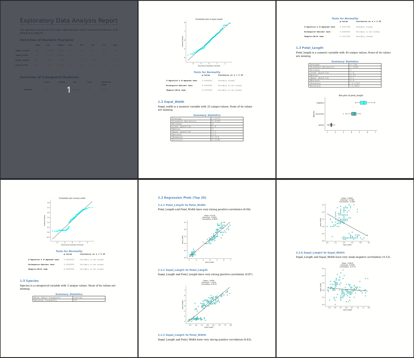
A Python program to help automate the exploratory data analysis and reporting process.

Input data is analyzed using pandas and SciPy. Graphs are plotted using matplotlib. The results are then nicely packaged as a Word (.docx) document using python-docx.

Installation

You can install the package from PyPI using:

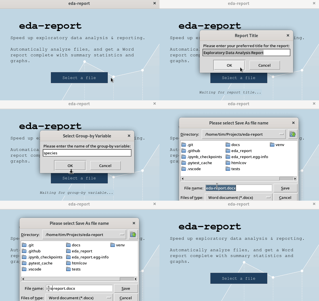
pip install eda-report

Basic Usage

1. Graphical User Interface

The eda-report command launches a graphical window to help select a csv/excel file to analyze:

eda-report

You'll be prompted to set a report title, group-by/target variable (optional), graph color and output filename; after which the contents of the input file are analyzed, and the results saved in a Word (.docx) document.

NOTE: For help with Tk - related issues, consider visiting TkDocs.

2. Command Line Interface

$ eda-report -i iris.csv -o iris-report.docx
Analyze variables:  100%|███████████████████████████████████| 5/5
Plot variables:     100%|███████████████████████████████████| 5/5
Bivariate analysis: 100%|███████████████████████████████████| 6/6 pairs.
[INFO 02:12:22.146] Done. Results saved as 'iris-report.docx'

$ eda-report -h
usage: eda-report [-h] [-i INFILE] [-o OUTFILE] [-t TITLE] [-c COLOR]
                  [-g GROUPBY]

Automatically analyze data and generate reports. A graphical user interface
will be launched if none of the optional arguments is specified.

optional arguments:
  -h, --help            show this help message and exit
  -i INFILE, --infile INFILE
                        A .csv or .xlsx file to analyze.
  -o OUTFILE, --outfile OUTFILE
                        The output name for analysis results (default: eda-
                        report.docx)
  -t TITLE, --title TITLE
                        The top level heading for the report (default:
                        Exploratory Data Analysis Report)
  -c COLOR, --color COLOR
                        The color to apply to graphs (default: cyan)
  -g GROUPBY, -T GROUPBY, --groupby GROUPBY, --target GROUPBY
                        The variable to use for grouping plotted values. An
                        integer value is treated as a column index, whereas a
                        string is treated as a column label.

3. Interpreter Session

>>> eda_report.summarize(iris_data)

                  Summary Statistics for Numeric features (4)
                  -------------------------------------------
                count     avg  stddev  min  25%   50%  75%  max  skewness  kurtosis
  sepal_length    150  5.8433  0.8281  4.3  5.1  5.80  6.4  7.9    0.3149   -0.5521
  sepal_width     150  3.0573  0.4359  2.0  2.8  3.00  3.3  4.4    0.3190    0.2282
  petal_length    150  3.7580  1.7653  1.0  1.6  4.35  5.1  6.9   -0.2749   -1.4021
  petal_width     150  1.1993  0.7622  0.1  0.3  1.30  1.8  2.5   -0.1030   -1.3406

                Summary Statistics for Categorical features (1)
                -----------------------------------------------
                    count unique     top freq relative freq
            species   150      3  setosa   50        33.33%


                        Pearson's Correlation (Top 20)
                        ------------------------------
      petal_length & petal_width -> very strong positive correlation (0.96)
     sepal_length & petal_length -> very strong positive correlation (0.87)
      sepal_length & petal_width -> very strong positive correlation (0.82)
      sepal_width & petal_length -> moderate negative correlation (-0.43)
       sepal_width & petal_width -> weak negative correlation (-0.37)
      sepal_length & sepal_width -> very weak negative correlation (-0.12)

Check out the documentation for more features and details.