reproduce OutbreakTools example using ggtree
This example is presented in vignette of OutbreakTools.
library(OutbreakTools)
data(FluH1N1pdm2009)
attach(FluH1N1pdm2009)

x <- new("obkData", individuals = individuals, dna = FluH1N1pdm2009$dna,
         dna.individualID = samples$individualID, dna.date = samples$date,
         trees = FluH1N1pdm2009$trees)

p <- plotggphy(x, ladderize = TRUE, branch.unit = "year",
               tip.color = "location", tip.size = 3, tip.alpha = 0.75)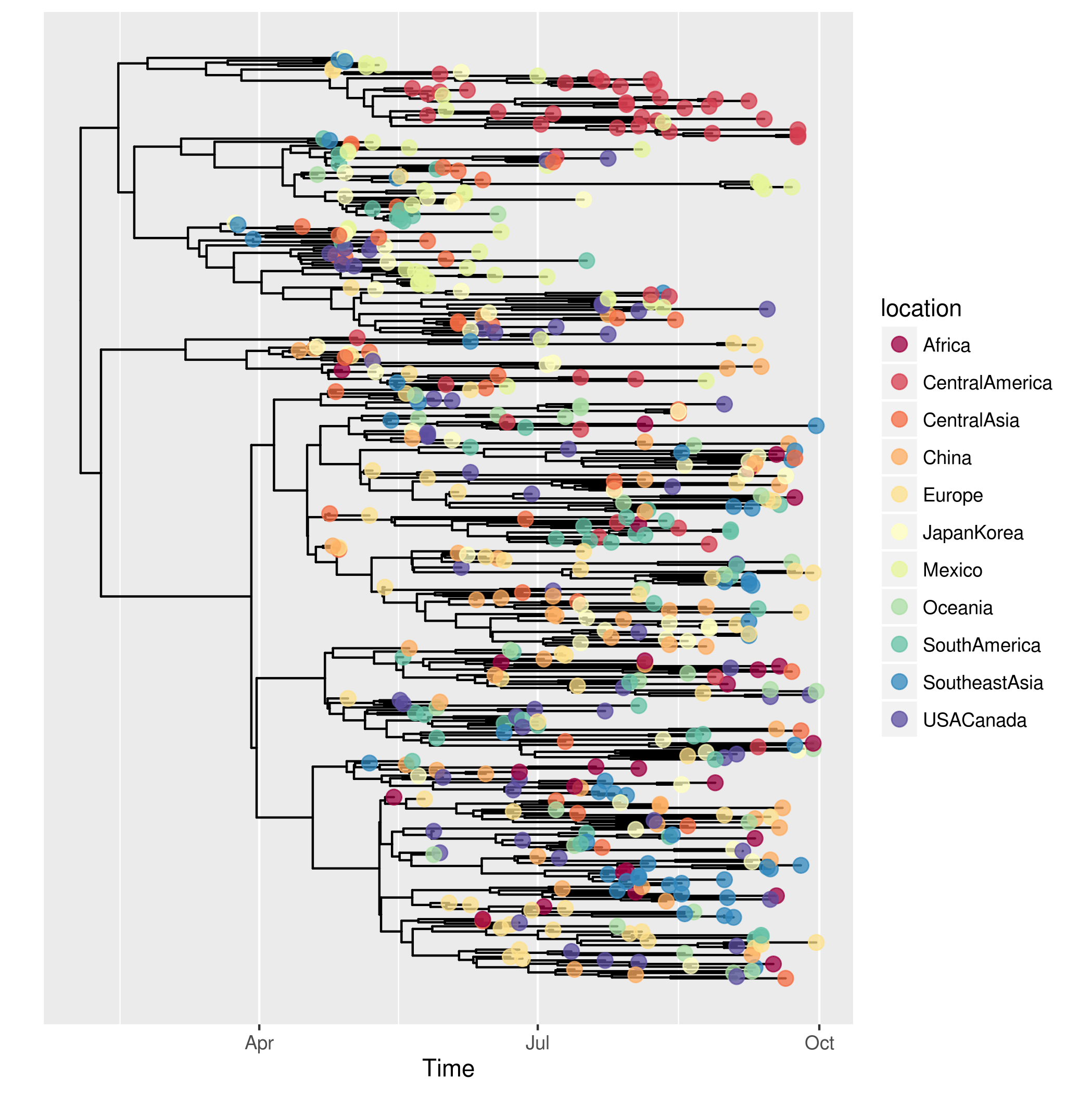
In this figure, it use Date for x-axis and the tree was annotated with Location. In an epidemic, time and location that of the virus sampled is important information and plotggphy is designed for viewing such information.
In ggtree, it's very easy to reproduce such figure by adding a layer of location information.
library(ggtree)

draw_OutbreakTools_ggtree <- function(x) {
    tree <- x@trees[[1]]
    g <- ggtree(tree, right=T, mrsd="2009-09-30", as.Date=TRUE) + theme_tree2()
    g <- g + theme(panel.grid.major = element_line(color="grey"),
                   panel.grid.major.y=element_blank())

    ## extract location info
    meta.df <- x@dna@meta
    meta.df <- data.frame(taxa=rownames(meta.df), meta.df)
    loc <- x@individuals
    loc <- data.frame(individualID=rownames(loc), loc)
    meta_loc <- merge(meta.df, loc, by="individualID")
    meta_loc <- meta_loc[,-1]

    ## attach additional information to tree view via %<+% operator
    ## that was created in ggtree
    g <- g %<+% meta_loc

    g + geom_tippoint(aes(color=location), size=3, alpha=.75) +
        theme(legend.position="right") +
            scale_color_brewer("location", palette="Spectral")
}

draw_OutbreakTools_ggtree(x)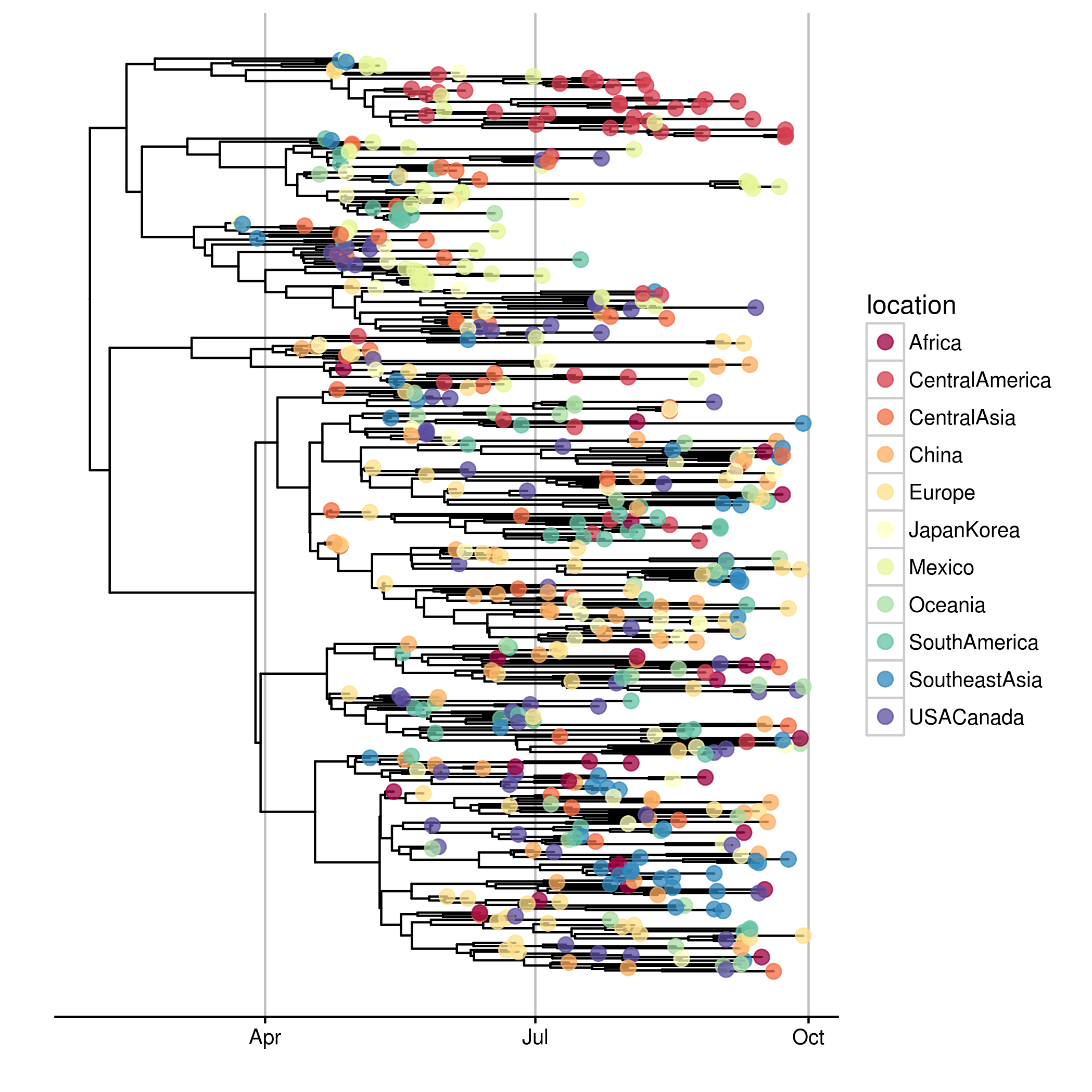
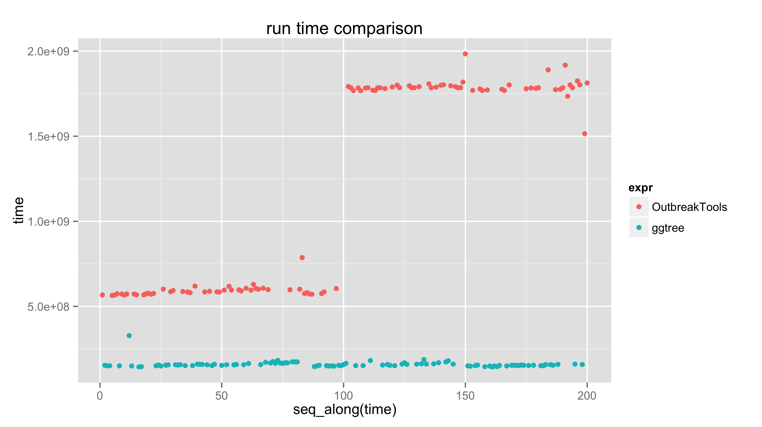
require(microbenchmark)

bm <- microbenchmark(
    OutbreakTools = plotggphy(x, ladderize = TRUE, branch.unit = "year",
        tip.color = "location", tip.size = 3, tip.alpha = 0.75),
    ggtree = draw_OutbreakTools_ggtree(x),
    times=100L
    )

print(bm)
## Unit: milliseconds
##           expr      min       lq      mean   median        uq       max neval
##  OutbreakTools 564.0195 585.7710 1225.8299 1767.713 1784.8457 1984.3352   100
##         ggtree 144.2246 151.7099  159.3318  155.200  160.9121  328.2016   100

qplot(y=time, data=bm, color=expr)  + ggtitle("run time comparison")