MCMCChains.jl

Implementation of Julia types for summarizing MCMC simulations and utility functions for diagnostics and visualizations.

Example

The following simple example illustrates how to use Chain to visually summarize a MCMC simulation:

using MCMCChains
using StatsPlots

theme(:ggplot2)

# Define the experiment
n_iter = 500
n_name = 3
n_chain = 2

# experiment results
val = randn(n_iter, n_name, n_chain) .+ [1, 2, 3]'
val = hcat(val, rand(1:2, n_iter, 1, n_chain))

# construct a Chains object
chn = Chains(val)

# visualize the MCMC simulation results
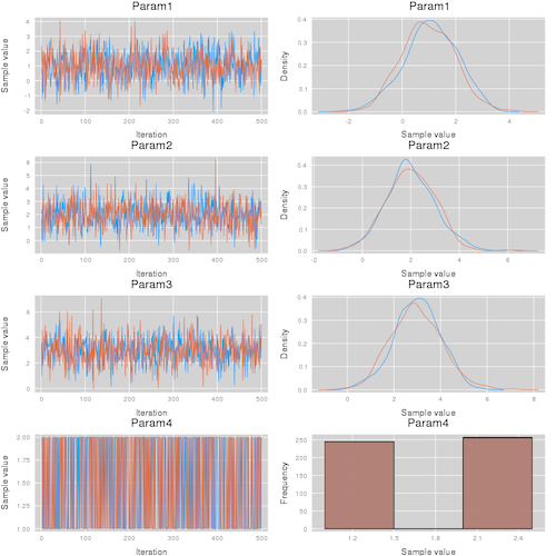
p1 = plot(chn)
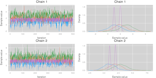
p2 = plot(chn, colordim = :parameter)

This code results in the visualizations shown below. Note that the plot function takes the additional arguments described in the Plots.jl package.

Summarize parameters	Summarize chains
plot(chn; colordim = :chain)	plot(chn; colordim = :parameter)

Manual

Chains type

# construction of a Chains object with no names
Chains(
    val::AbstractArray{A,3};
    start::Int=1,
    thin::Int=1,
    evidence = 0.0,
    info=NamedTuple(),
)

Chains(
    val::AbstractArray{A,3},
    parameter_names::AbstractVector,
    name_map = (parameters = parameter_names,);
    start::Int=1,
    thin::Int=1,
    evidence = 0.0,
    info=NamedTuple(),
)

# Indexing a Chains object
chn = Chains(...)
chn_param1 = chn[:,2,:] # returns a new Chains object for parameter 2
chn[:,2,:] = ... # set values for parameter 2

Parameter Names

Chains can be constructed with parameter names, like so:

# 500 samples, 5 parameters, two chains.
val = rand(500,5, 2)

chn = Chains(val, ["a", "b", "c", "d", "e"])

By default, parameters will be given the name :param_i, where i is the parameter number.

Rename Parameters

Parameter names can be changed with the function replacenames, which accepts a Chains object and pairs of old and new parameter names. Note that replacenames creates a new Chains object that shares the same underlying data.

chn = Chains(
	rand(100, 5, 5),
	["one", "two", "three", "four", "five"],
	Dict(:internals => ["four", "five"])
)

# Set "one" and "five" to uppercase.
chn2 = replacenames(chn,  "one" => "ONE", "five" => "FIVE")

# Alternatively you can provide a dictionary.
chn3 = replacenames(chn, Dict("two" => "TWO", "four" => "FOUR"))

Sections

Chains parameters are sorted into sections that represent groups of parameters. By default, every chain contains a :parameters section, to which all unassigned parameters are assigned to. Chains can be assigned a named map during construction:

chn = Chains(val,
  ["a", "b", "c", "d", "e"],
  Dict(:internals => ["d", "e"]))

The set_section function returns a new Chains object:

chn2 = set_section(chn, Dict(:internals => ["d", "e"]))

Any parameters not assigned will be placed into :parameters.

Calling display(chn) provides the following output:

Chains MCMC chain (500×5×2 Array{Float64,3}):

Iterations        = 1:500
Thinning interval = 1
Chains            = 1, 2
Samples per chain = 500
parameters        = a, b, c
internals         = d, e

Summary Statistics
  parameters      mean       std   naive_se      mcse         ess      rhat
      Symbol   Float64   Float64    Float64   Float64     Float64   Float64

           a    0.4930    0.2906     0.0092    0.0095   1044.0585    1.0030
           b    0.5148    0.2875     0.0091    0.0087    992.1013    0.9984
           c    0.5046    0.2899     0.0092    0.0087    922.6449    0.9987

Quantiles
  parameters      2.5%     25.0%     50.0%     75.0%     97.5%
      Symbol   Float64   Float64   Float64   Float64   Float64

           a    0.0232    0.2405    0.4836    0.7530    0.9687
           b    0.0176    0.2781    0.5289    0.7605    0.9742
           c    0.0258    0.2493    0.5071    0.7537    0.9754

Note that only a, b, and c are being shown. You can explicity retrieve an array of the summary statistics and the quantiles of the :internals section by calling describe(chn; sections = :internals), or of all variables with describe(chn; sections = nothing). Many functions such as plot or gelmandiag support the sections keyword argument.

Groups of parameters

By convention, MCMCChains assumes that parameters with names of the form "name[index]" belong to one group of parameters called :name. You can access the names of all parameters in a chain that belong to the group :name by running

namesingroup(chain, :name)

If the chain contains a parameter of name :name it will be returned as well.

The function group(chain, :name) returns a subset of the chain chain with all parameters in the group :name.

The get Function

MCMCChains provides a get function designed to make it easier to access parameters get(chn, :P) returns a NamedTuple which can be easy to work with.

Example:

val = rand(500, 5, 1)
chn = Chains(val, ["P[1]", "P[2]", "P[3]", "D", "E"]);

x = get(chn, :P)

Here's what x looks like:

(P = (Union{Missing, Float64}[0.349592; 0.671365; … ; 0.319421; 0.298899], Union{Missing, Float64}[0.757884; 0.720212; … ; 0.471339; 0.5381], Union{Missing, Float64}[0.240626; 0.987814; … ; 0.980652; 0.149805]),)

You can access each of the P[. . .] variables by indexing, using x.P[1], x.P[2], or x.P[3].

get also accepts vectors of things to retrieve, so you can call x = get(chn, [:P, :D]). This looks like

(P = (Union{Missing, Float64}[0.349592; 0.671365; … ; 0.319421; 0.298899], Union{Missing, Float64}[0.757884; 0.720212; … ; 0.471339; 0.5381], Union{Missing, Float64}[0.240626; 0.987814; … ; 0.980652; 0.149805]),
 D = Union{Missing, Float64}[0.648963; 0.0419232; … ; 0.54666; 0.746028])

Note that x.P is a tuple which has to be indexed by the relevant index, while x.D is just a vector.

Convergence Diagnostics functions

Discrete Diagnostic

Options for method are [:weiss, :hangartner, :DARBOOT, MCBOOT, :billinsgley, :billingsleyBOOT]

discretediag(c::Chains; frac=0.3, method=:weiss, nsim=1000)

Gelman, Rubin, and Brooks Diagnostics

gelmandiag(c::Chains; alpha=0.05, mpsrf=false, transform=false)

Geweke Diagnostic

gewekediag(c::Chains; first=0.1, last=0.5, etype=:imse)

Heidelberger and Welch Diagnostics

heideldiag(c::Chains; alpha=0.05, eps=0.1, etype=:imse)

Raftery and Lewis Diagnostic

rafterydiag(c::Chains; q=0.025, r=0.005, s=0.95, eps=0.001)

Rstar Diagnostic

Rstar diagnostic described in https://arxiv.org/pdf/2003.07900.pdf. Note that the use requires MLJ and MLJModels to be installed.

Usage:

using MLJ, MLJModels

chn ... # sampling results of multiple chains

# select classifier used to compute the diagnostic
classif = @load XGBoostClassifier

# estimate diagnostic
Rs = rstar(classif, chn)
R = mean(Rs)

# visualize distribution
using Plots
histogram(Rs)

See ? rstar for more details.

Model Selection

Deviance Information Criterion (DIC)

chn ... # sampling results
lpfun = function f(chain::Chains) # function to compute the logpdf values
    niter, nparams, nchains = size(chain)
    lp = zeros(niter + nchains) # resulting logpdf values
    for i = 1:nparams
        lp += map(p -> logpdf( ... , x), Array(chain[:,i,:]))
    end
    return lp
end
DIC, pD = dic(chn, lpfun)

Plotting

# construct a plot
plot(c::Chains, seriestype = (:traceplot, :mixeddensity))

# construct trace plots
plot(c::Chains, seriestype = :traceplot)

# or for all seriestypes use the alternative shorthand syntax
traceplot(c::Chains)

# construct running average plots
meanplot(c::Chains)

# construct density plots
density(c::Chains)

# construct histogram plots
histogram(c::Chains)

# construct mixed density plots
mixeddensity(c::Chains)

# construct autocorrelation plots
autocorplot(c::Chains)

# make a cornerplot (requires StatPlots) of parameters in a Chain:
corner(c::Chains, [:A, :B])

Saving and Loading Chains

Like any Julia object, a Chains object can be saved using Serialization.serialize and loaded back by Serialization.deserialize as identical as possible. Note, however, that in general this process will not work if the reading and writing are done by different versions of Julia, or an instance of Julia with a different system image. You might want to consider JLSO for saving metadata such as the Julia version and the versions of all packages installed as well.

# Save a chain.
using Serialization
serialize("chain-file.jls", chn)

# Read a chain.
chn2 = deserialize("chain-file.jls")

Exporting Chains

A few utility export functions have been provided to convers Chains objects to either an Array or a DataFrame:

# Several examples of creating an Array object:
Array(chns)
Array(chns[:s])
Array(chns, [:parameters])
Array(chns, [:parameters, :internals])

# By default chains are appended. This can be disabled
# using the append_chains keyword argument:
Array(chns, append_chains=false)

# This will return an `Array{Array, 1}` object containing
# an Array for each chain.

# A final option is:
Array(chns, remove_missing_union=false)

# This will not convert the Array columns from a
# `Union{Missing, Real}` to a `Vector{Real}`.

Similarly, for DataFrames:

DataFrame(chns)
DataFrame(chns[:s])
DataFrame(chns, [:parameters])
DataFrame(chns, [:parameters, :internals])
DataFrame(chns, append_chains=false)
DataFrame(chns, remove_missing_union=false)

See also ?DataFrame and ?Array for more help.

Sampling Chains

MCMCChains overloads several sample methods as defined in StatsBase:

# Sampling `n` samples from the chain `a`. Optionally
# weighting the samples using `wv`.
sample([rng], a, [wv::AbstractWeights], n::Integer)

# As above, but supports replacing and ordering.
sample([rng], a, [wv::AbstractWeights], n::Integer; replace=true,
  ordered=false)

See also ?sample for additional help. Alternatively, you can construct and sample from a kernel density estimator using the KernelDensity package:

using KernelDensity

# Construct a kernel density estimator
c = kde(Array(chn[:s]))

# Generate 10000 weighted samples from the grid points
chn_weighted_sample = sample(c.x, Weights(c.density), 100000)

License Notice

Note that this package heavily uses and adapts code from the Mamba.jl package licensed under MIT License, see License.md.