Workflow
TODO: Elaborate on TDoA, FDoA
TODO: Fix references
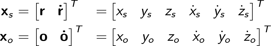
Satellite and observer state vectors are represented in Earth-Centered Inertial (ECI) coordinate frame:
The slant (line-of-sight) component of the range rate is then given by the dot product between the velocity difference and line-of-sight unit vector:
![]()
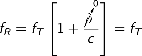
The observed Doppler shift can then be expressed as follows:
![]()
where ![]() and
and ![]() denote received and transmitted frequencies and c denotes the speed of light. If the transmitted frequency is unknown, it can be obtained by observing the Doppler shift at the time and recording the frequency at the time of closest approach (TOCA) when the slant range rate is zero:
denote received and transmitted frequencies and c denotes the speed of light. If the transmitted frequency is unknown, it can be obtained by observing the Doppler shift at the time and recording the frequency at the time of closest approach (TOCA) when the slant range rate is zero:
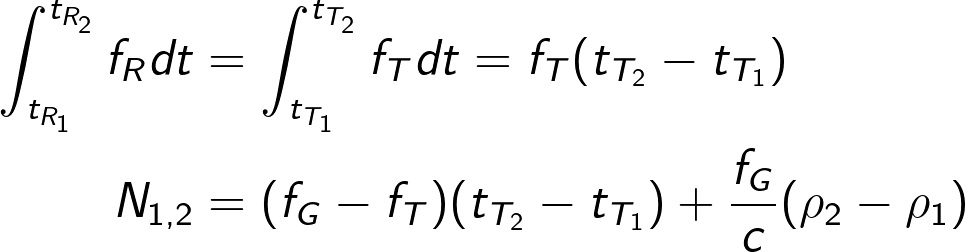
Another measurement model that also uses Doppler Shift is so-called Doppler Counts. When a transmitted frequency arrives at the ground station, it is mixed with some ground reference frequency ![]() and the number of of cycles for a certain time period of this mixed frequency
and the number of of cycles for a certain time period of this mixed frequency ![]() is recorded:
is recorded:
![]()
A separate note should be made on timing notations - as it takes some finite time for signal to reach the observer, both satellite and observer are moving during this time period, ![]() designates the transmission time at timestep
designates the transmission time at timestep ![]() and
and ![]() - reception, accordingly. The relationship between transmission and reception time are as follows:
- reception, accordingly. The relationship between transmission and reception time are as follows:
![]()
where ![]() is the distance between the satellite at transmission time and the observer at the reception time and
is the distance between the satellite at transmission time and the observer at the reception time and ![]() is the time of flight. By noting the previous equation the doppler counts equation can be further expanded:
is the time of flight. By noting the previous equation the doppler counts equation can be further expanded:
![]()
Also note that:
Additionally, for a short period of time, the previous equation can be rearranged as:
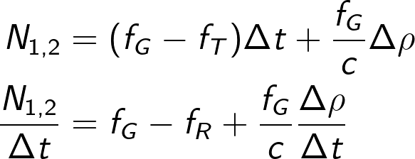
By setting the ground reference frequency ![]() , the equation is further simplified, giving the measurement model:
, the equation is further simplified, giving the measurement model:
![]()
The proposed orbit determination routine for this project is expected to be split into three main parts:
- Initial position estimate through multilateration
- Initial orbit determination
- Sequential/Batch estimation using direct (Doppler shift) or generated (multilaterated position) measurement
Two common techniques for multilateration, or object location estimation using the difference in distance or velocities of sensors with respect to the object include Time Differential of Arrival (TDoA) and Frequency Differential of Arrival (FDoA). In TDoA, the location of the object is estimated from the difference in distances between the sensors and the object at known timestamps, while the FDoA exploits the Doppler shift caused by the relative movement of the sensors and the object.
TODO: Elaborate on TDoA
The time difference in signal arrival is directly proportional to the distance difference between the emitter and the sensors.
![]()
In TDoA approach, observer positions are to be known while emitter position is the unknown variable to be found. The ranges between the observer and the emitter are determined using the estimate of the time it takes for signal to travel between the emitter and the observer. In order to obtain the position estimate for the signal source, the following system of equations can be used [ref]:
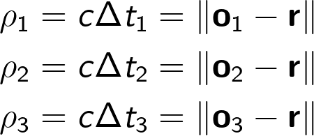
However, the actual time it takes for the signal to reach the receiver is unknown, but relative formulation of the above system is possible:
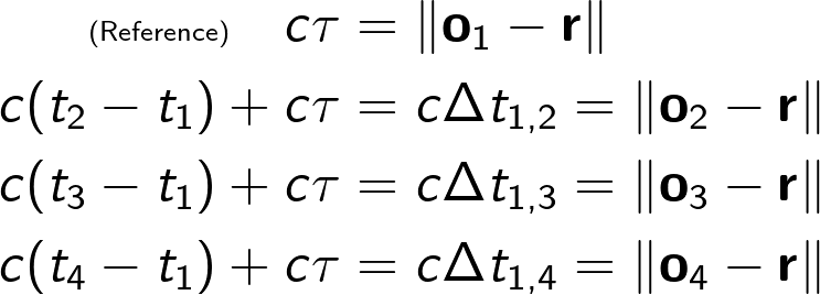
In relative formulation, one receiver serves as a reference, and receives a signal with some unknown offset ![]() . Then, the rest of the receivers obtain the signal with some time differentce
. Then, the rest of the receivers obtain the signal with some time differentce ![]() . As additional unknown variable is introduced, it is now necessary to use at least four stations in order to solve this system of equations - three variables for source position coordinates and one for
. As additional unknown variable is introduced, it is now necessary to use at least four stations in order to solve this system of equations - three variables for source position coordinates and one for ![]() offset. After solving this system of equations, the position estimate of the signal source is obtained.
offset. After solving this system of equations, the position estimate of the signal source is obtained.
A simple 2D TDoA example is shown in the picture below.

In the following scenario, three sensors and emitter are present on a 2D plane. As can be seen, two sensors are enough to find curve intersection with single positional ambiguity. Third sensor curve intersection coincides with the first two curves intersections.
In a three-dimensional scenario, observations from three stations are required to obtain position estimate when signal timing is available. In case of relative formulation, at least four stations are necessary. Second ambigous location can be neglected using sanity check (e.g. position above the Earth surface).
TODO: Look into FDoA in detail, elaborate on FDoA
FDoA, also known as Differential Doppler technique operates in a similar manner to TDoA, however, in this case, Doppler shift is used. The frequency difference between two points is directly proportional to the radial velocities differences:
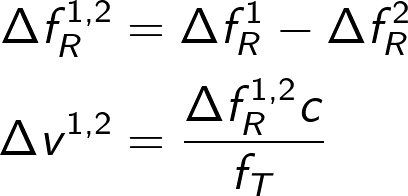
where ![]() denotes the received frequency difference at n-th sensor.
denotes the received frequency difference at n-th sensor.
There are numerous techniques for initial orbit determination. Given the fact, that positional estimate is obtained through multilateration, it is only necessary to calculate the velocity component of the state vector.
Herrick-Gibbs initial orbit determination method calculates a velocity vector give three consequtive positional measurements with their corresponding timestamps. It uses Taylor series expansion to obtain a velocity vector for middle measurement. The summary of the method is presented below:

Consequtively, from three positional measurements a single full-state orbital estimate can be obtained, that can be further used as a separate measurement or initial estimate input for a sequential tracking method.
So far, three variables can be used as input for sequential or batch estimation:
- Doppler shift
- Orbiting object dynamic system is unobservable through Doppler measurements only
- Multilaterated position
- Observable, no velocity estimate
- Initial orbit estimate from Herrick-Gibbs Method
- Observable, velocity estimate, thus can be used in propagation
Given full-state initial estimate from Herrick-Gibbs IOD method, Kalman Filter is plug-and-play online solution for sequential estimation.
For offline solution, batch filter can be provided both with sequences of positional and full-state measurements.
The accuracy of the multilaterated solution greatly depends on spatial separation of the receiving stations as well as timing accuracy of the sensors.
- Fundamentals of Astrodynamics and Applications
- Fundametals of Astrodynamics
- Statistical Orbit Determination
- Satellite Orbits: Models, Methods and Applications
- The Doppler Determination of Orbits
- Determination of Orbital Elements and Refraction Effects from Single Pass Doppler Observations
- Method of Doppler Data Processing for Orbit Determination
- Rapid Determination of Satellite Orbits from Doppler Data