Classification Using Logistic Regression

Attract customers with promotions.

---

List of contents

• Description
• Descriptive Statistical Analysis
• Feature Engineering
• Feature Selection
• Develop Model
• Statistical Evaluation
• Final Product
• About the Author

---

Description

This project has an objective to help fintech companies to classify members who will get promos using logistic regression. The data provided is raw data in the form of csv which is data from 50,000 users with 12 variables first_open, dayofweek, hour, liked etc. members who will get promos are members who are most likely not subscribed to premium services. This is intended that with the promo they will be interested in using the premium features.

Technologies

• Python
• Logistic Regression
• K fold cross validation

Back To The Top

---

Descriptive Statistical Analysis

Descriptive statistics is a statistical analysis that provides a general description of the characteristics of each variable, thereby providing useful information.

Importing Libraries and data

import numpy as np
import pandas as pd
import matplotlib.pyplot as plt
import seaborn as sns

#import data set
dataku = pd.read_csv('data_fintech.csv')

Creating a Histogram

#ringkasan data
ringkasan = dataku.describe()
tipe_data = dataku.dtypes

#revisi kolom num screen
dataku['screen_list'] = dataku.screen_list.astype(str)+','
#membuat kolom perhitungan koma
dataku['num_screens'] = dataku.screen_list.str.count(',')
dataku.drop(columns=['numscreens'],inplace =True)

#konversi hour dari object ke integer
dataku.hour[1]
dataku.hour = dataku.hour.str.slice(1,3).astype(int)

#drop semua colom yang bukan angka 
dataku_numerik = dataku.drop(columns=['user', 'first_open','screen_list'
                                      ,'enrolled_date'], inplace = False)
#membuat histogram
sns.set()
plt.suptitle('Overview Data')
for i in range(0,dataku_numerik.shape[1]):
    plt.subplot(3,3,i+1)
    figure = plt.gca()
    figure.set_title(dataku_numerik.columns.values[i])
    jumlah_bin = np.size(dataku_numerik.iloc[:,i].unique())
    plt.hist(dataku_numerik.iloc[:,i], bins=jumlah_bin)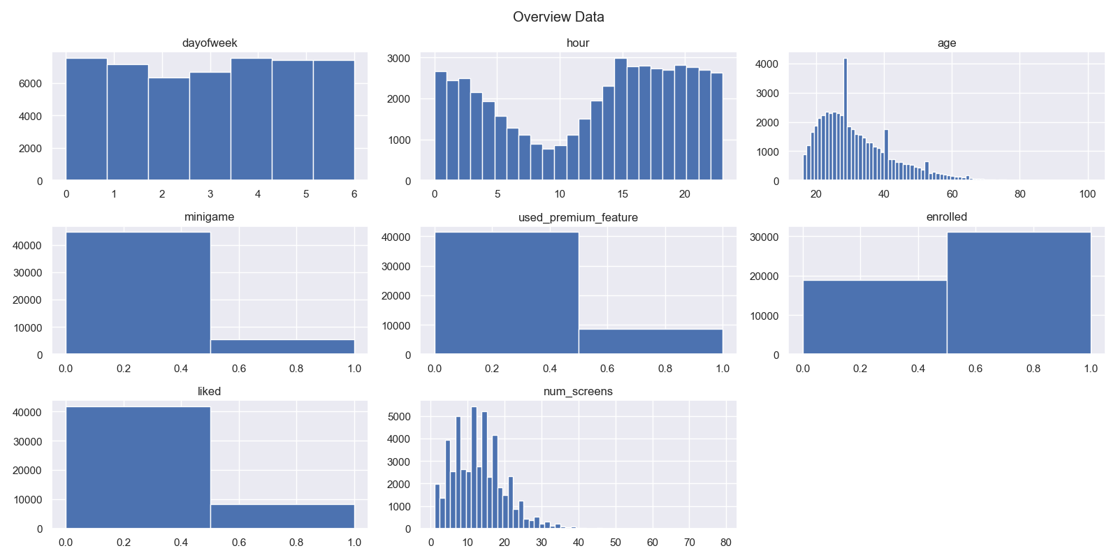

From the collection of histograms of each variable, it can be seen that the variables age and num_screens have an abnormal or skewed distribution.

Finding Correlation of Variables to Enrolled Decision

korelasi = dataku_numerik.drop(columns=['enrolled'],inplace=False).corrwith(dataku_numerik.enrolled)
korelasi.plot.bar('korelasi variable terhadap keputusan enrolled')

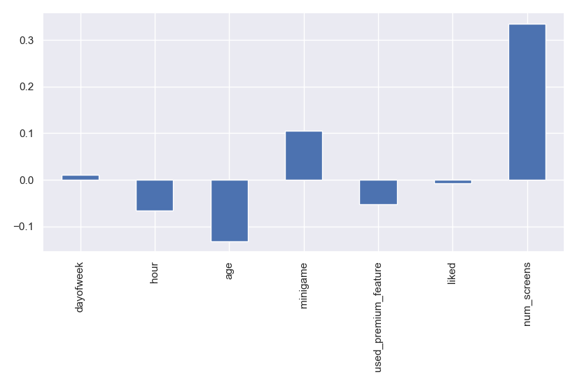
Of the 7 variables that have been changed to numeric form. The num_screens variable has the highest correlation, which means that the more users access the number of screens, the greater the possibility of users to enroll premium features. However, the correlation percentage is only 0.3, meaning it is not so strong that it is not a noise variable that can dim other variables.

Creating a Heatmap Between Variables

#membuat heatmap antar variable
matriks_korelasi = dataku_numerik.drop(columns=['enrolled'],inplace=False).corr()
sns.heatmap(matriks_korelasi, cmap='Reds')

#membuat heatmap custom
#buat matriks mask
mask = np.zeros_like(matriks_korelasi, dtype = np.bool)
mask[np.triu_indices_from(mask)] =True
#heatmap custom
ax = plt.axes()
cmapku = sns.diverging_palette(200,0,as_cmap=True)
sns.heatmap(matriks_korelasi,cmap=cmapku,mask=mask,linewidths=0.5,center=0,square=True)
ax=plt.suptitle('matriks korelasi antar variabel')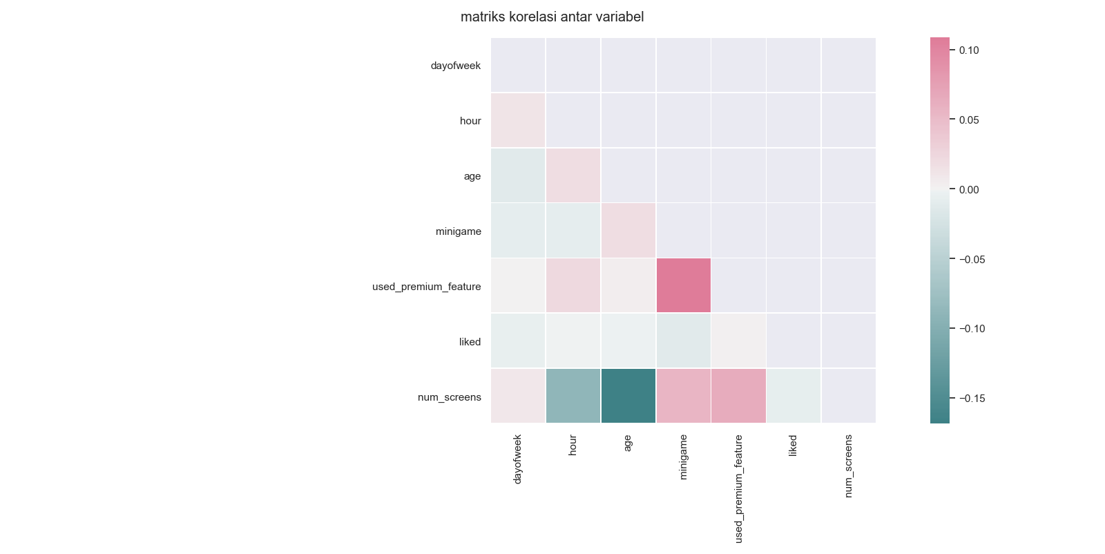

In this heat map, each correlation between one variable and another variable is displayed more widely.

Back To The Top

---

Feature Engineering

In the analysis above, it is known that there are several variables/features that are not normally distributed or skewed. This non-normally distributed data is caused by data that does not represent the population or what we call noise. So Feature Engineering is needed to eliminate noise.

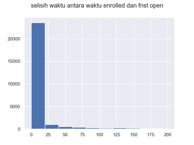
The data shows that from 0-25 is a representation of the population. The difference is the time the user subscribed and the time they first opened the application. In this case, the author took the data range 0-50 as the population to train the model.

Repairing Data and Removing Noise

#proses parsing
from dateutil import parser
dataku.first_open = [parser.parse(i) for i in dataku.first_open]
dataku.enrolled_date = [parser.parse(i) if isinstance(i,str) else i for i in dataku.enrolled_date]
dataku['selisih'] = (dataku.enrolled_date - dataku.first_open).astype('timedelta64[h]') 

#membuat histogram dataku['selisih']
plt.hist(dataku.selisih.dropna(), range =[0,200])
plt.suptitle('selisih waktu antara waktu enrolled dan frist open')
plt.show()
#memfilter nilai selisih yang lebih dari 50 jam karena tidak merepresentasikan populasi
dataku.loc[dataku.selisih>50,'enrolled']=0

The parsing process is used to analyze, or in this case to change/repair the first_open column which is still in text/string form into numeric form.

Membreakdown Layar Layar Yang di Akses Oleh User

In the dataset (my data) we have a screen_list column, in that column we select the most frequently accessed screens. Therefore, a second data set is needed, namely the top_screens dataset provided by the fintech party.

#mengimport data top screen

top_screens = pd.read_csv('top_screens.csv')
top_screens = np.array(top_screens.loc[:,'top_screens'])
#mencopy dataku
dataku2 = dataku.copy()

#membuat kolom topscreen
for layar in top_screens:
    dataku2[layar] = dataku2.screen_list.str.contains(layar).astype(int)

for layar in top_screens:
    dataku2['screen_list'] = dataku2.screen_list.str.replace(layar+',','')

#menghitung layar selain top screen
dataku2['lainya'] = dataku2.screen_list.str.count(',')

top_screens.sort()

At this stage the data is clean from noise and has been changed to the correct format for the next stage.

Back To The Top

---

Feature Selection

In Feature Engineering we have broken down the screens that are frequently accessed by users. However, some of the top_screens lists provided by the fintech party have similarities such as the loan screen there is loan, loan 2, loan 3 etc. Likewise for the saving, credit and cc screens, then with Feature selection we combine similar screens.

Combining Multiple Similar Variables

# teknik funneling. penyederhanaan variable yang mirip

layar_loan = ['Loan',
              'Loan2',
              'Loan3',
              'Loan4']
dataku2['jumlah_loan'] = dataku2[layar_loan].sum(axis=1)
dataku2.drop(columns=layar_loan, inplace = True)

layar_saving = ['Saving1',
                'Saving2',
                'Saving2Amount',
                'Saving4',
                'Saving5',
                'Saving6',
                'Saving7',
                'Saving8',
                'Saving9',
                'Saving10']
dataku2['jumlah_Saving'] = dataku2[layar_saving].sum(axis=1)
dataku2.drop(columns=layar_saving, inplace = True)


layar_credit= ['Credit1',
               'Credit2',
               'Credit3',
               'Credit3Container',
               'Credit3Dashboard']
dataku2['jumlah_credit'] = dataku2[layar_credit].sum(axis=1)
dataku2.drop(columns=layar_credit, inplace = True)

layar_cc =['CC1',
           'CC1Category',
           'CC3']
dataku2['jumlah_cc'] = dataku2[layar_cc].sum(axis=1)
dataku2.drop(columns=layar_cc,inplace=True)

#mendefisinikan var dependen
var_enrolled = np.array(dataku2['enrolled'])

#menghilangkan kolom redundant
dataku2.drop(columns = ['user','first_open','enrolled','screen_list',
                        'enrolled_date'],inplace =True)
dataku2.drop(columns =['selisih'],inplace = True)

Now all the data needed to perform the modeling is ready.

Back To The Top

---

Develop Model

To train a model that aims to classify users, the author tried to use the method logistic egression. This method is a general linear model used for binomial regression.

#membagi training set dan test set

from sklearn.model_selection import train_test_split
X_train,X_test,y_train, y_test = train_test_split(np.array(dataku2),var_enrolled,
                                                  test_size = 0.2,
                                                  random_state = 111)
#menghapus variabel kosong
X_train = np.delete (X_train,27,1)
X_test = np.delete (X_test,27,1)

#scalling. standarisasi data

from sklearn.preprocessing import StandardScaler
sc_X = StandardScaler()
X_train = sc_X.fit_transform(X_train)
X_test = sc_X.fit_transform(X_test)

#LOGISTIC REGRESSION

from sklearn.linear_model import LogisticRegression
classifier = LogisticRegression(random_state=0, solver='liblinear',
                                penalty='l1')

classifier.fit(X_train, y_train)

#mencoba membuat prediksi pada X_test
y_pred = classifier.predict(X_test)

#melihat evaluasi dengan confussion matrix
from sklearn.metrics import confusion_matrix, accuracy_score, classification_report
cm= confusion_matrix(y_test, y_pred)

It turns out that in column 27 there is a variable whose entire number is 0. So we just remove this variable.

Back To The Top

---

Statistical Evaluation

Calculating Accuracy Score

evaluasi = accuracy_score(y_test, y_pred)
print('akurasi:{:.2f}'.format(evaluasi*100))

akurasi:76.32

Confusion Matrix Visualization With Seaborn

cm_label= pd.DataFrame(cm, columns=np.unique(y_test),
                       index= np.unique(y_test))
cm_label.index.name='aktual'
cm_label.columns.name='prediksi'
sns.heatmap(cm_label, annot= True, cmap='Reds',fmt='g') 

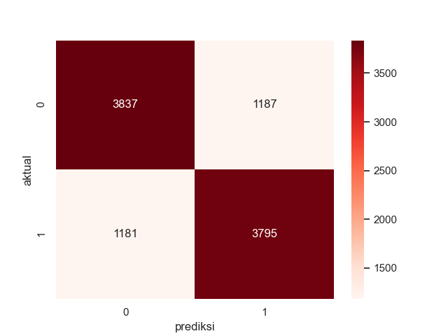
The confusion matrix diagram shows that the logistic regression model is able to predict 3837 unenrolled users correctly and 1187 incorrectly, and predict 3795 enrolled users correctly and 1181 incorrectly.

Validation With 10 Fold Cross Validation

#validasi dengan 10 fold cross validation
from sklearn.model_selection import cross_val_score
accuracies = cross_val_score(estimator=classifier,X=X_train,y=y_train, cv=10)

#melihat mean dan standart deviasi
accuracies.mean()
accuracies.std()

print('akurasi logistic regresi ={:.2f}% +/- {:.2f}%'.format(accuracies.mean()*100,accuracies.std()*100))

akurasi logistic regresi =76.58% +/- 0.79%

This model is a model that predicts decisions based on user behavior so that the accuracy is quite high, above 75%.

Back To The Top

Produk Final

What the company needs is a list of users who will be given a promo or not. So the KPI is a list of users who will be given a promo.

Create a Suggested List of People Who Should Get the Promo

#membuat daftar saran orang yang akan mendapatkan promo
#mencopy dataku
dataku2 = dataku.copy()
var_enrolled = dataku2['enrolled']
from sklearn.model_selection import train_test_split
X_train,X_test,y_train, y_test = train_test_split(dataku2,var_enrolled,
                                                  test_size = 0.2,
                                                  random_state = 111)

train_id = X_train['user']
test_id = X_test['user']

#menggabungkan
y_pred_series = pd.Series(y_test).rename('asli',inplace =True)
hasil_akhir = pd.concat([y_pred_series,test_id],axis=1).dropna()
hasil_akhir['prediksi'] = y_pred
hasil_akhir = hasil_akhir[['user','asli','prediksi']].reset_index(drop=True)

Because in the feature selection process we discard the user column because we only need the numeric column. So to track the user we re-copy my data and divide it with train_test_split with the same random state. so that at the end of the process the list desired by the company is available.

Back To The Top

---

Tentang Penulis

Hi, I'm Albara, I'm an industrial engineering student at the Islamic University of Indonesia who is interested in data science. If you want to contact me, you can send a message to the following link.

• Twitter - @albara_bimakasa
• Email - [email protected]

Back To The Top