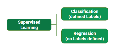
Supervised Machine Learning - Regression

• Supervised learning is the types of machine learning in which machines are trained using well "labelled" training data, and on basis of that data, machines predict the output. The labelled data means some input data is already tagged with the correct output.

• In supervised learning, the training data provided to the machines work as the supervisor that teaches the machines to predict the output correctly. It applies the same concept as a student learns in the supervision of the teacher.

• Supervised learning is a process of providing input data as well as correct output data to the machine learning model. The aim of a supervised learning algorithm is to find a mapping function to map the input variable(x) with the output variable(y).

How Supervised Learning Works?

In supervised learning, models are trained using labelled dataset, where the model learns about each type of data. Once the training process is completed, the model is tested on the basis of test data (a subset of the training set), and then it predicts the output.

The working of Supervised learning can be easily understood by the below example and diagram:

Steps Involved in Supervised Learning:

• First Determine the type of training dataset.
• Collect/Gather the labelled training data.
• Split the training dataset into training dataset, test dataset, and validation dataset.
• Determine the input features of the training dataset, which should have enough knowledge so that the model can accurately predict the output.
• Determine the suitable algorithm for the model, such as support vector machine, decision tree, etc.
• Execute the algorithm on the training dataset. Sometimes we need validation sets as the control parameters, which are the subset of training datasets.
• Evaluate the accuracy of the model by providing the test set. If the model predicts the correct output, which means our model is accurate.

Types of supervised Machine learning Algorithms:

Regression

• Regression analysis is a statistical method to model the relationship between a dependent (target) and independent (predictor) variables with one or more independent variables.
• In Regression, we plot a graph between the variables which best fits the given datapoints, using this plot, the machine learning model can make predictions about the data. In simple words, "Regression shows a line or curve that passes through all the datapoints on target-predictor graph in such a way that the vertical distance between the datapoints and the regression line is minimum." The distance between datapoints and line tells whether a model has captured a strong relationship or not.

Terminologies Related to the Regression Analysis:

• Dependent Variable: The main factor in Regression analysis which we want to predict or understand is called the dependent variable. It is also called target variable.
• Independent Variable: The factors which affect the dependent variables or which are used to predict the values of the dependent variables are called independent variable, also called as a predictor.
• Outliers: Outlier is an observation which contains either very low value or very high value in comparison to other observed values. An outlier may hamper the result, so it should be avoided.
• Multicollinearity: If the independent variables are highly correlated with each other than other variables, then such condition is called Multicollinearity. It should not be present in the dataset, because it creates problem while ranking the most affecting variable.
• Underfitting and Overfitting: If our algorithm works well with the training dataset but not well with test dataset, then such problem is called Overfitting. And if our algorithm does not perform well even with training dataset, then such problem is called underfitting.

Types of Regression

• Simple Linear Regression

• Multiple Linear Regression

• Polynomial Regression

• Support Vector Regression

• Decision Tree Regression

• Random Forest Regression

---

Simple Linear Regression

The Simple Linear Regression model can be represented using the below equation:

y= b0 + b1.x1

Implementation of Simple Linear Regression Algorithm using Python

Problem Statement

Here we are taking a dataset that has two variables: salary (dependent variable) and experience (Independent variable).

	YearsExperience	Salary
0	1.1	39343.0
1	1.3	46205.0
2	1.5	37731.0
3	2.0	43525.0
4	2.2	39891.0
5	2.9	56642.0
...	...	...
25	9.0	105582.0
26	9.5	116969.0
27	9.6	112635.0
28	10.3	122391.0
29	10.5	121872.0

The goals of this problem is:

• We want to find out if there is any correlation between these two variables
• We will find the best fit line for the dataset.
• How the dependent variable is changing by changing the independent variable.

Step-1: Data Pre-processing

Data Pre-processing

Step-2: Fitting the Simple Linear Regression to the Training Set:

we will import the LinearRegression class of the linear_model library from the scikit learn. After importing the class, we are going to create an object of the class named as a regressor.

from sklearn.linear_model import LinearRegression
regressor = LinearRegression()
regressor.fit(X_train, y_train)

Step: 3. Prediction of test set result:

We will create a prediction vector y_pred, and x_pred, which will contain predictions of test dataset, and prediction of training set respectively.

#Prediction of Test and Training set result
y_pred= regressor.predict(x_test)
x_pred= regressor.predict(x_train)

Step: 4. visualizing the Training set results:

• we will use the scatter() function of the pyplot library, which we have already imported in the pre-processing step. The scatter () function will create a scatter plot of observations.

• In the x-axis, we will plot the Years of Experience of employees and on the y-axis, salary of employees.

• Now, we need to plot the regression line, so for this, we will use the plot() function of the pyplot library. In this function, we will pass the years of experience for training set, predicted salary for training set x_pred, and color of the line(Blue).

• Next, we will give the title for the plot. So here, we will use the title() function of the pyplot library and pass the name ("Salary vs Experience (Training Dataset)".

• After that, we will assign labels for x-axis and y-axis using xlabel() and ylabel() function.

plt.scatter(X_train, y_train, color = 'red')
plt.plot(X_train, x_pred, color = 'blue')
plt.title('Salary vs Experience (Training set)')
plt.xlabel('Years of Experience')
plt.ylabel('Salary')
plt.show()

Step: 5. visualizing the Test set results:

plt.scatter(X_test, y_test, color = 'red')
plt.plot(X_test, y_pred, color = 'blue')
plt.title('Salary vs Experience (Test set)')
plt.xlabel('Years of Experience')
plt.ylabel('Salary')
plt.show()

Step: 6. Combining all the steps:

Now, in the end, we can combine all the steps together to make our complete code more understandable.

Complete Code

If You want To Run The Code Then You Can Use Google Colab

NOTE : Before running the Program upload This Dataset.

---

Multiple Linear Regression

• In Simple Linear Regression, where a single Independent/Predictor(X) variable is used to model the response variable (Y).
• But there may be various cases in which the response variable is affected by more than one predictor variable; for such cases,
• The Multiple Linear Regression algorithm is used.

MLR equation:

• In Multiple Linear Regression, the target variable(Y) is a linear combination of multiple predictor variables x1, x2, x3, ...,xn.
• Since it is an enhancement of Simple Linear Regression, so the same is applied for the multiple linear regression equation, the equation becomes:

Assumptions for Multiple Linear Regression:

• A linear relationship should exist between the Target and predictor variables.
• The regression residuals must be normally distributed.
• MLR assumes little or no multicollinearity (correlation between the independent variable) in data.

Implementation of Multiple Linear Regression model using Python:

Problem Description:

• We have a dataset of 50 start-up companies.
• This dataset contains five main information: R&D Spend, Administration Spend, Marketing Spend, State, and Profit for a financial year.

	R&D Spend	Administration	Marketing Spend	State	Profit
0	165349.20	136897.80	471784.10	New York	192261.83
1	162597.70	151377.59	443898.53	California	191792.06
2	153441.51	101145.55	407934.54	Florida	191050.39
3	144372.41	118671.85	383199.62	New York	182901.99
4	142107.34	91391.77	366168.42	Florida	166187.94
5	131876.90	99814.71	362861.36	New York	156991.12
...	...	...	...	...	...
45	1000.23	124153.04	1903.93	New York	64926.08
46	1315.46	115816.21	297114.46	Florida	49490.75
47	0.00	135426.92	0.00	California	42559.73
48	542.05	51743.15	0.00	New York	35673.41
49	0.00	116983.80	45173.06	California	14681.40

• Our goal is to create a model that can easily determine which company has a maximum profit, and which is the most affecting factor for the profit of a company.

Step-1: Data Pre-processing Step:

Data Pre-processing

Step: 2- Fitting our MLR model to the Training set:

from sklearn.linear_model import LinearRegression
regressor = LinearRegression()
regressor.fit(X_train, y_train)

Step: 3- Prediction of Test set results:

y_pred = regressor.predict(X_test)
np.set_printoptions(precision=2)
print(np.concatenate((y_pred.reshape(len(y_pred),1), y_test.reshape(len(y_test),1)),1))

We can also check the score for training dataset and test dataset.

print('Train Score: ', regressor.score(X_train, y_train))
print('Test Score: ', regressor.score(X_test, y_test))

Step: 4. Combining all the steps:

Now, in the end, we can combine all the steps together to make our complete code more understandable.

Complete Code

If You want To Run The Code Then You Can Use Google Colab

NOTE : Before running the Program upload This Dataset.

---

Polynomial Regression

• Polynomial Regression is a regression algorithm that models the relationship between a dependent(y) and independent variable(x) as nth degree polynomial.

• It is also called the special case of Multiple Linear Regression in ML. Because we add some polynomial terms to the Multiple Linear regression equation to convert it into Polynomial Regression.
• It is a linear model with some modification in order to increase the accuracy.
• The dataset used in Polynomial regression for training is of non-linear nature.
• It makes use of a linear regression model to fit the complicated and non-linear functions and datasets.

Note:

A Polynomial Regression algorithm is also called Polynomial Linear Regression because it does not depend on the variables, instead, it depends on the coefficients, which are arranged in a linear fashion.

Implementation of Polynomial Regression using Python :

Problem Description:

• There is a Human Resource company, which is going to hire a new candidate. The candidate has told his previous salary 160K per annum, and the HR have to check whether he is telling the truth or bluff.
• So to identify this, they only have a dataset of his previous company in which the salaries of the top 10 positions are mentioned with their levels.

	Position	Level	Salary
0	Business Analyst	1	45000
1	Junior Consultant	2	50000
2	Senior Consultant	3	60000
3	Manager	4	80000
4	Country Manager	5	110000
5	Region Manager	6	150000
6	Partner	7	200000
7	Senior Partner	8	300000
8	C-level	9	500000
9	CEO	10	1000000

• By checking the dataset available, we have found that there is a non-linear relationship between the Position levels and the salaries.
• Our goal is to build a Bluffing detector regression model, so HR can hire an honest candidate. Below are the steps to build such a model.

Step-1: Data Pre-processing Step:

Data Pre-processing

Step: 2- Training the Linear Regression model on the whole dataset V/S Training the Polynomial Regression model on the whole dataset

Training the Linear Regression model on the whole dataset :

from sklearn.linear_model import LinearRegression
lin_reg = LinearRegression()
lin_reg.fit(X, y)

Training the Polynomial Regression model on the whole dataset :

from sklearn.preprocessing import PolynomialFeatures
poly_reg = PolynomialFeatures(degree = 4)
X_poly = poly_reg.fit_transform(X)
lin_reg_2 = LinearRegression()
lin_reg_2.fit(X_poly, y)

Step: 3- Visualising the Linear Regression results V/S Visualising the Polynomial Regression results

Visualising the Linear Regression results :

plt.scatter(X, y, color = 'red')
plt.plot(X, lin_reg.predict(X), color = 'blue')
plt.title('Truth or Bluff (Linear Regression)')
plt.xlabel('Position Level')
plt.ylabel('Salary')
plt.show()

Visulalising the Polynomial Regression results :

plt.scatter(X, y, color = 'red')
plt.plot(X, lin_reg_2.predict(poly_reg.fit_transform(X)), color = 'blue')
plt.title('Truth or Bluff (Polynomial Regression)')
plt.xlabel('Position level')
plt.ylabel('Salary')
plt.show()

Step: 4- Predicting a new result with Linear Regression V/S Predicting a new result with Polynomial Regression

Predicting a new result with Linear Regression :

lin_reg.predict([[6.5]])

Predicting a new result with Polynomial Regression :

lin_reg_2.predict(poly_reg.fit_transform([[6.5]]))

Step: 5. Combining all the steps:

Now, in the end, we can combine all the steps together to make our complete code more understandable.

Complete Code

If You want To Run The Code Then You Can Use Google Colab

NOTE : Before running the Program upload This Dataset.

---

Support Vector Regression (SVR)

• The problem of regression is to find a function that approximates mapping from an input domain to real numbers on the basis of a training sample.

- Consider the end of yellow boundary as the decision boundary and the middle line within yello region as the hyperplane. Our objective, when we are moving on with SVR, is to basically consider the points that are within the decision boundary line. Our best fit line is the hyperplane that has a maximum number of points.

• The first thing that we’ll understand is what is the decision boundary.Consider these lines as being at any distance, say ‘a’, from the hyperplane. So, these are the lines that we draw at distance ‘+a’ and ‘-a’ from the hyperplane. This ‘a’ in the text is basically referred to as epsilon.

• Assuming that the equation of the hyperplane is as follows:

Y = wx+b (equation of hyperplane)

Then the equations of decision boundary become:

wx+b= +a
wx+b= -a

Thus, any hyperplane that satisfies our SVR should satisfy:

-a < Y- wx+b < +a

• Our main aim here is to decide a decision boundary at ‘a’ distance from the original hyperplane such that data points closest to the hyperplane or the support vectors are within that boundary line.

• Hence, we are going to take only those points that are within the decision boundary and have the least error rate, or are within the Margin of Tolerance. This gives us a better fitting model.

Implementation of Polynomial Regression using Python :

Problem Description:

• There is a Human Resource company, which is going to hire a new candidate. The candidate has told his previous salary 160K per annum, and the HR have to check whether he is telling the truth or bluff.
• So to identify this, they only have a dataset of his previous company in which the salaries of the top 10 positions are mentioned with their levels.

	Position	Level	Salary
0	Business Analyst	1	45000
1	Junior Consultant	2	50000
2	Senior Consultant	3	60000
3	Manager	4	80000
4	Country Manager	5	110000
5	Region Manager	6	150000
6	Partner	7	200000
7	Senior Partner	8	300000
8	C-level	9	500000
9	CEO	10	1000000

• By checking the dataset available, we have found that there is a non-linear relationship between the Position levels and the salaries.
• Our goal is to build a Bluffing detector regression model, so HR can hire an honest candidate. Below are the steps to build such a model.

Step-1: Data Pre-processing Step:

Data Pre-processing

Step-2: Training the SVR model on the whole dataset

from sklearn.svm import SVR
regressor = SVR(kernel = 'rbf')
regressor.fit(X, y)

Step-3: Predicting a new result

sc_y.inverse_transform(regressor.predict(sc_X.transform([[6.5]])).reshape(-1,1))

Step-4: Visualising the SVR results

plt.scatter(sc_X.inverse_transform(X), sc_y.inverse_transform(y), color = 'red')
plt.plot(sc_X.inverse_transform(X), sc_y.inverse_transform(regressor.predict(X).reshape(-1,1)), color = 'blue')
plt.title('Truth or Bluff (SVR)')
plt.xlabel('Position level')
plt.ylabel('Salary')
plt.show()

Step-5: Visualising the SVR results (for higher resolution and smoother curve)

X_grid = np.arange(min(sc_X.inverse_transform(X)), max(sc_X.inverse_transform(X)), 0.1)
X_grid = X_grid.reshape((len(X_grid), 1))
plt.scatter(sc_X.inverse_transform(X), sc_y.inverse_transform(y), color = 'red')
plt.plot(X_grid, sc_y.inverse_transform(regressor.predict(sc_X.transform(X_grid)).reshape(-1,1)), color = 'blue')
plt.title('Truth or Bluff (SVR)')
plt.xlabel('Position level')
plt.ylabel('Salary')
plt.show()

Step-6: Combining all the steps:

Now, in the end, we can combine all the steps together to make our complete code more understandable.

Complete Code

If You want To Run The Code Then You Can Use Google Colab

NOTE : Before running the Program upload This Dataset.

---

---

Created And Coded By:

Pritam Das

🔗 Feedback

If you have any feedback, please reach out to me at