-
Notifications
You must be signed in to change notification settings - Fork 0
Additional data

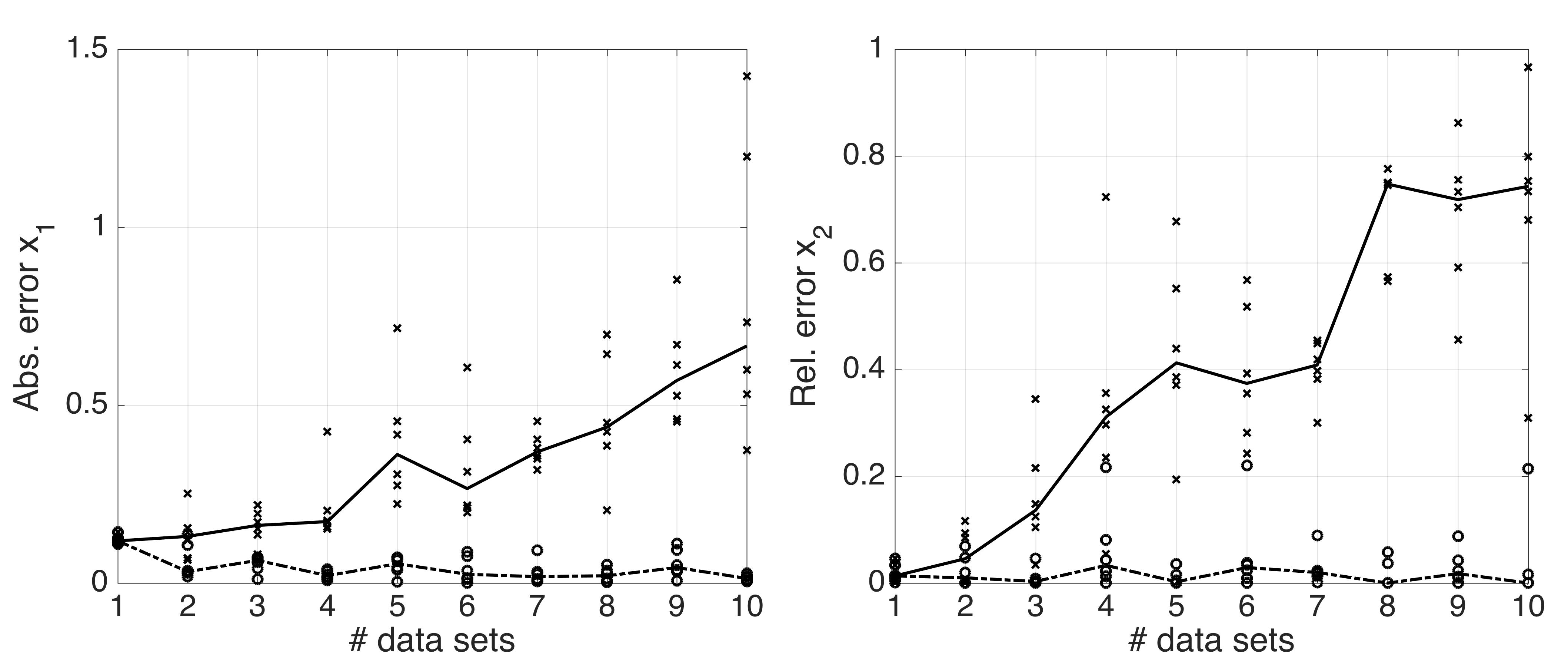
Figure: maximum (cross) and minimum (circles) deviations for x1 and x2 with median profiles (solid and dashed lines, respectively).
We have performed optimization with up to ten data sets with 5 features and 300 samples. Each DATA scatter was drawn from a standard normal distribution Ν(0,1). MODEL function generates data for each data set (again, 5 features and 300 samples) by varying two parameters of the standard normal distribution, i.e. N(x1,x2). We fix all other configurations of the optimization. The results are shown in the figure above.
Since we know the true values of x1 and x2 (0.0, and 1.0, respectively), we can assess the optimization performance as a function of number of data sets by calculating max and min deviations from the true values across the data sets in a series of similar optimization runs (here, 6 runs per case). One can see from the figure that the median profile for the maximum deviation increases with the number of data sets.
Note such increase in the estimate deviations is for the given optimization configuration. For example, we have verified that if we allow for larger number of iterations, we will not observe the increase (data not shown) as a function of number of data sets, since the optimization for any number of data sets between 1 and 10 is equally good given the longer search time. To observe the increase one would need to increase the number of data sets even more. Thus, it is purely a characteristic of the optimization routine.
Some morphological clones (best-fit SSM) obtained during Espoo maple studies (see Potapov et al., GigaScience, 2017, available online)

Figure: The Espoo maple QSM is in the middle, the best-fit SSMs are named by date, each having three clones presented.
The Espoo maple studies reported in Potapov et al., GigaScience, 2017, available online)
morpho-clones.zip archive contains the simulated data and all necessary information to repeat the simulations reported in the paper.
The QSM data are located in EspooData.mat file. It contains several reconstruction models of the target tree, but we used only the model 1. Make sure the file is loaded into the MATLAB's workspace by:
load('EspooData.mat');The above command will create a variable called EspooData, which is accessed by the
function BayesForest. To run a specific simulation with the configuration in, say,
input.txt file just type at the MATLAB prompt:
BayesForest('input.txt')All configuration files are located in the folders named by date and time. For example:
- The rosette-shape tree simulation is in 12.11.2016_18.22
- The best-fit SSM simulation is in 6.1.2017_19.15
Other simulations are available with their description in the lab-book README.
The usual simulation time is long (up to several days on a modest computer). One can use simpler test runs for the Toolbox: see the tutorial.
Besides MATLAB one needs LPFG. LPFG is a simulator based on the L+C language (L-system paradigm in C++ expressions). The simulator is available in the VLAB (Unix) or L-studio (Windows) packages from the Algorithmic Botany website. The version used in this study was 4.4.0-2424 for 64-bit Mac OS (OS X version 10.11.6 El Capitan).
LPFG simulates the growth of a tree (self-organizing tree model, from sot-dist-1.2.8.zip file).
BayesForest Toolbox
The Inverse Problems Research Group, Tampere University of Technology
Copyright 2013-2017 Ilya Potapov, contribute and distribute freely