


auto-period-finder is an autocorrelation function (ACF) based seasonality periods automatic finder for univariate time series.
To install the latest version of auto-period-finder, simply run:
pip install auto-period-finderStart by loading a timeseries dataset with a frequency. We can use co2 emissions sample dataset from statsmodels
from statsmodels.datasets import co2
data = co2.load().data
You can resample the data to whatever frequency you want.
data = data.resample("ME").mean().ffill()Use AutoPeriodFinder to find the list of seasonality periods based on ACF.
from auto_period_finder import AutoPeriodFinder
period_finder = AutoPeriodFinder(data)
periods = period_finder.fit()
You can also find the most prominent period either ACF-wise:
strongest_period_acf = period_finder.fit_find_strongest_acf()or variance-wise:
strongest_period_var = period_finder.fit_find_strongest_var()You can learn more about calculating seasonality component through variance from here.
This project is built and published using Poetry. To setup development environment for this project you can follow these steps:
- First, you need to install Python of one of the compatible versions indicated above.
- Install Poetry. You can follow this guide and use their official installer.
- Navigate to the root folder and install dependencies in a virtual environment:
poetry install- If everything worked properly, you should have
auto-period-finder-geinoPPi-py3.10environment activated. You can verify this by running:
poetry env list- You can run tests using the command:
poetry run pytest- To export the list detailed list of dependencies, run the following command:
poetry self add poetry-plugin-export
poetry export --output requirements.txtAn easy and quick way to find seasonality periods of a univariate time series is to check its autocorrelation function (ACF) and look for specific charecteristics in lag values that we will detail in a second. You can read more information about time series ACF here, but intuitively, An autocorrelation coefficient
Simply put, given a univariate time series
$1 \lt k \leq \frac{\lvert T \rvert}{2}$ - Autocorrelation coefficients
$r_q$ are local maxima where$q \in {k, 2k, 3k, ...}$ -
$\forall p \in P, \forall n \in \mathbb{N}, k \neq n \times p$ , where$P$ is the list of already found periods.
The list of such
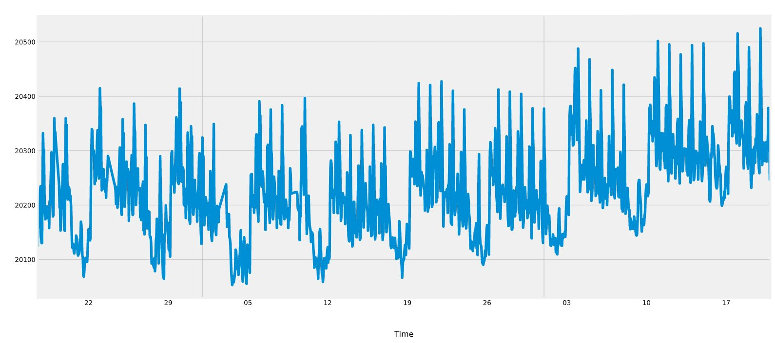
Now let's look at the corresponding ACF for the time series above:
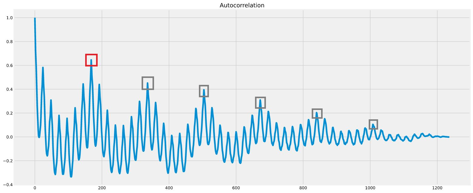
You can see that the autocorrelation coefficient for lag value 168 hours (i.e. one week) is a local maximum (red-border square). Similarly, autocorrelation coefficient for lag values that are multiples of 168 (gray-border squares). We can therefore conclude that this time series has a weekly seasonality period.
- The first condition is needed because a seasonality period cannot neither be 1 (a trivial case), nor greater than half the length of the target time series (by definition, a seasonality has to manifest itself at least twice in a given time series).
- The third condition favors eliminating redundant seasonality periods that are multiples of each others. The algorithm does allow, however, finding seasonality periods that divide already found seasonality periods.
- The periods detection uses
argmaxon the ACF to select seasonality period candidates before checking they satisfy the conditions discussed above. Therefore, the list of seasonality periods are returned in the descending order of their corresponding ACF coefficients.
- [1] Hyndman, R.J., & Athanasopoulos, G. (2021) Forecasting: principles and practice, 3rd edition, OTexts: Melbourne, Australia. OTexts.com/fpp3. Accessed on 12-25-2023.