ISOMAP

Non-Linear Dimension Reduction

TL;DR

ISOMAP is a non-linear dimension reduction method to reduce the size and complexity of a dataset, projecting it onto a new plain. This method is useful for datasets with non-linear structure, where PCA and MDS will not be appropriate.

Questions:

• What is this method? ISOMAP, a Non-Linear Dimension Reduction method

• What does it do? When should I use it? This projects the dataset into a reduce plain that shrinks the dimension while keeping most of the information from the data. It essentially transforms the space in which the data is represented. This can be used to shrink the size of a non-linear high-dimensional dataset like images, or as a pre-processing step for clustering.

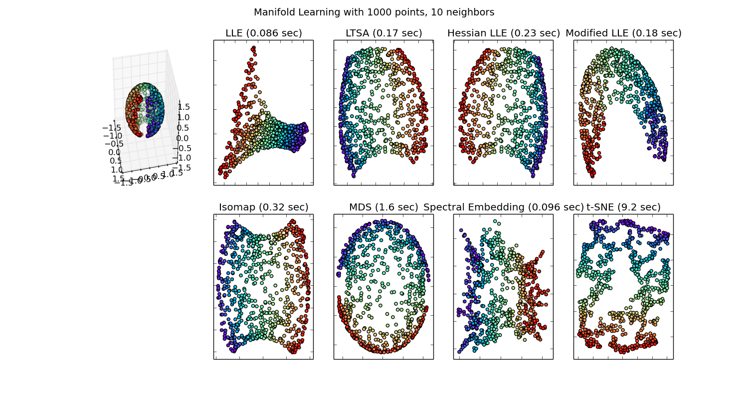
• What are the alternatives and how does this one compare? Alternatives are PCA, and MDS for linear data and t-SNE for non-linear. There are actually many Manifold learning methods which can be seen here and newly published in 2018, UMAP
  

• What are it’s failure modes (when not to use) and how to you diagnose them? ISOMAP is dependent on thresholding or KNN in it's first step to create an adjacency matrix, which can be sensitive to noisy or sparse data. In addition, it can become computationally expensive.

• How do I call this (is there are module/package? git repo? other?) Implementations of ISOMAP can found in most programming languages, but to start exploring I suggest Sci-Kit Learn for Python.

Dimension Reduction

Dimension reduction is used in when we have very high-dimensional data, which is to say many columns or features. This appears often in image processing and biometric processing. In many cases, we want to reduce the complexity, size of the data, or improve interpretation. We can use dimension reduction methods to achieve this using methods like PCA for linear data and ISOMAP for non-linear data.

TL;DR:

• Feature Selection
• Feature Projection
• Size Reduction
• Visual Charting in 2 or 3 dimensions

When would someone use dimension reduction?

• Under-determined system, more features than samples (Regularization)
• Data is too large for system, cannot afford more compute
• Reduce size of data to decrease time to solve, time sensative
• Removal of multi-collinearity
• Can lead to improved model accuracy for regression and classification Rico-Sulayes, Antonio (2017)
• Visualize the relationship between the data points when reduced to 2D or 3D

Algorithm

There are three steps to the ISOMAP algorithm.

Step 1 Adjacency & Distance Matrices

Since our data has a non-linear form we will view our data as a network. This will allow us to have some flexibility around the shape of our data and connect data that is "close". There are two ways to create your edges between your nodes

The first way to create edges is to use KNN and connect each node to the closest K neighbors. Note that we do not need to use Euclidean distance but can and should try many different distances to see which has the best results for your particular dataset. Often in high dimensions, Euclidean distance breaks down and we must start searching elsewhere. See links at the bottom for information on different distance metrics.

Alternatively, you can use threshold to decide your edges. If two points are within your distance threshold, then they are connected, otherwise the distance between the two nodes is set to infinity. You can tune your threshold so that each node has some minimum number of connections, which is what we'll use in our example.

Image from Georgia Tech ISyE 6740, Professor Yao Xie

Once you have your adjacency matrix, we'll create our distance matrix which has the shortest path between each point and every other point. This matrix will be symmetric since we are not creating a directed graph. This is the main difference between ISOMAP and a linear approach. We'll allow the path to travel through the shape of the data showing the points are related even though they might not actually be "close" regarding your distance metric.

For example, if our adjacency matrix is

[[0   0.2 INF],
 [0.2 0   0.7]
 [INF 0.7   0]]

Then our distance matrix D would be

[[0   0.2 0.9],
 [0.2 0   0.7]
 [0.9 0.7   0]]

Because 1 can reach 3 through 2. This can be implemented as such

def make_adjacency(data, dist_func="euclidean", eps=1):
   n, m = data.shape
   dist = cdist(data.T, data.T, metric=dist_func)
   adj =  np.zeros((m, m)) + np.inf
   bln = dist < eps  # who is connected?
   adj[bln] = dist[bln]
   short_path = graph_shortest_path(adj)

   return short_path

Step 2 Centering Matrix

Now we'll create the centering matrix that will be use to modify the distance matrix D we just created.

Now, we'll use this centering matrix on our distance matrix D to create our kernel matrix, K

Step 3 Eigenvalues & Eigenvectors

Finally, we take an eigenvalue decomposition of the kernel matrix K. The largest N (in our case 2) eigenvalues and their corresponding eigenvectors are the projections of our original data into the new plain. Since eigenvectors are all linearly independent thus, we will avoid collision.

def isomap(d, dim=2):
    n, m = d.shape
    h = np.eye(m) - (1/m)*np.ones((m, m))
    d = d**2
    c = -1/(2*m) * h.dot(d).dot(h)
    evals, evecs = linalg.eig(c)
    idx = evals.argsort()[::-1]
    evals = evals[idx[:dim]]
    evecs = evecs[:, idx[:dim]]
    z = evecs.dot(np.diag(evals**(-1/2)))

    return z.real

Example

In our example we'll take over 600 images, which are 64 x 64 and black & White, and project them into a two dimensional space. This project can be used to cluster or classify the images in another machine learning model.

If we use a linear method, like PCA, we will get a reduced result, but the relationship between the data is not clear the eye.

Now, by running Isomap, we can show the corresponding images by their projected point and see that after the projection, the points that are near each other are quite similar. So the direction the face is looking, that information was carried through the projection. Now this smaller dataset, from (684 x 4096) to (684 x 2) can be used as input to a clustering method like K-means.

Additional Resources

• Sci-kit Learn
• Original Paper
• Another Example
• t-SNE A great alternative
• More t-SNE Interactive visuals

Wiki articles:

• Nonlinear Dimensionality reduction
• Model Reduction
• Dimensionality Reduction

Different Distance Metrics

• Intuition - Math.net
• SciPy Distances
• Sci-Kit Learn

Unrelated but these guys in general are good.