MoBILAB

See Notes about current meetings and test data.

Mobilab is a multimodal data browser and motion capture data preprocessor for XDF format data.

Introduction

A new paradigm for human brain imaging, mobile brain/body imaging (MoBI), involves synchronous collection of human brain activity (via electroencephalography, EEG), behavior (via body motion capture, eye tracking, etc.) and environmental events (via scene and experimental event recording) to study the joint brain / body dynamics supporting natural human cognition, i.e., motivated human actions and interactions in natural 3-D environments (Makeig et al., 2009). Processing complex, concurrent, multi-modal, and multi-rate data streams requires a signal processing environment quite different from environments designed to process single-modality time series data.

MoBILAB Toolbox for MATLAB was designed in 2011 by Alejandro Ojeda with Nima Bigdley Shamlo, and Christian Kothe in consultation with Arnaud Delorme and Scott Makeig, to support the Mobile Brain/Body imaging (MoBI) paradigm (Makeig et al., 2009). Since then, the software has evolved from a simple plug-in that bridged multi-modal data collection systems with EEGLAB software environment (Delorme & Makeig, 2004), to a standalone, open source, cross platform toolbox operating on MATLAB (The Mathworks, Inc.) that supports analysis and visualization of any combination of synchronously recorded brain, body, behavioral, and environmental data, designed primarily to enable joint analyses of EEG, body motion, and other behavioral data streams.

To make working with concurrent data streams of different modalities as simple as possible, MoBILAB exploits object-oriented programming (oop) to ease supporting new data types. In contrast to the common practice of representing data streams as in-memory variables in MATLAB workspace, MoBILAB uses memory-mapped data files to make it possible to process data streams of virtually any size without requiring large amounts of random access memory (RAM) and without compromising performance. Currently MoBILAB includes classes designed for holding, analyzing and visualizing EEG, motion capture, eye tracking, and force plate data as well as for recorded audio and video. These classes include methods (functions acting on class properties) for filters, time derivatives, wavelet time-frequency decomposition, independent component analysis (ICA), principal component analysis (PCA), and realistic electrical forward head and inverse EEG source modeling.

References

Makeig S, Gramann K, Jung T-P, Sejnowski TJ, Poizner (2009). Linking brain, mind and behavior: The promise of mobile brain/body imaging (MoBI). International Journal of Psychophysiology 73:985-100.

Delorme A, Makeig S, EEGLAB: an open source toolbox for analysis of single-trial EEG dynamics including independent component analysis (2004) Journal of Neuroscience Methods 134:9-21.

A Ojeda, N Bigdely-Shamlo, S Makeig. MoBILAB: An open source toolbox for analysis and visualization of mobile brain/body imaging data. Frontiers in Human Neuroscience, 2014.

See also:

1. the EEGLAB Home pages,
2. the LabStreamingLayer software distribution, and
3. its mulitmodal, extensible XDF data format.

Shortcut to practical chapters

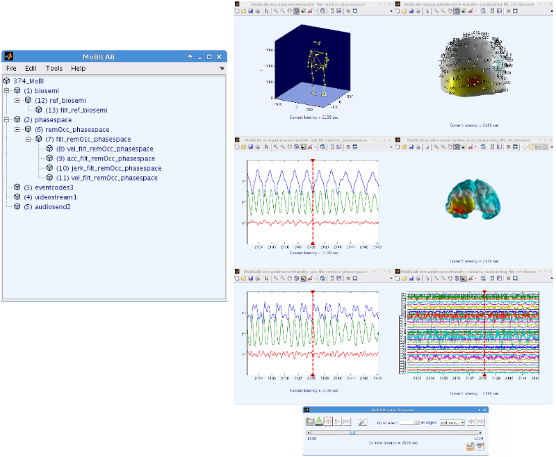
The following tutorials are available: Run MoBILAB from the MoBILAB GUI: MoBILAB operation Run MoBILAB from the Matlab command line: MoBILAB commands Head model module: https://github.com/aojeda/headModel

Download MoBILAB Toolbox

MoBILAB toolbox is hosted on GitHub: https://github.com/aojeda/mobilab

How to reference this software

If you use this toolbox please cite our paper.

MATLAB Object-Oriented Programming, an overview

The MATLAB language enables the creation of programs using both procedural and object-oriented techniques.

Procedural programming typically represents data as individual variables or field of a structure and implements operations as functions that take the variables as arguments. Programs typically call a sequence of functions, each one of which is passed data and then returns modified data. As functions become too large and complex, a common approach is to break them into smaller functions. However, as the number of functions becomes large, designing and managing the data passed to functions becomes difficult and error prone.

Object oriented programming or OOP tries to overcome this issue identifying commonalities, differences, and interacting pieces of the software and encapsulates them in classes. As a real-life system can be decomposed into objects (example: car -> engine -> fuel system -> oxygen sensor), one piece of software can be decoupled into modules defined by natural logical boundaries. These modules (objects) provide interfaces by means of which they can interact with other modules (other objects or functions).

For more information about MATLAB OOP see MATLAB reference.

OOP basic definitions

A class describes a set of objects with common characteristics. Objects are specific instances of a class as variable a may be from the built-in class single, double, or char (see example here). Objects from the same class may differ in the data contained in their properties but the functions defining how they operate on them and interact with external parameters may be common for all instances of a given class, these functions are called methods.

In MATLAB one might organize classes in hierarchies, this facilitates reusing the code and solutions to design problems that have been already solved. MoBILAB is been implemented using the following class hierarchies: 1) data sources: for importing data from different acquisition systems, 2) stream objects: for analysis of different types of MoBI data on continuous time, 3) epoch objects: for more traditional ERP analysis, and 4) stream browsers: for visualization and annotation of the different data-types.

Note for users not familiar with OOP: I heard somewhere a remark that I found very true -- paraphrased goes like this: It is OK if at first glance a new language looks alien to you -- every new language does until we get used to it (unless that language is Perl). Fortunately, MATLAB oop is much easier than Perl.

MoBILAB software architecture

MoBILAB software is built from three independent functional modules: 1) data-specific objects that "know" what to do with their data set, 2) a datasource object that reads different data formats (locally or remotely) and serves the independent files to the data-specific objects, and 3) an object called "mobilab" that lives in MATLAB's workspace, this object is in charge of controlling the GUI and drawing data-dependent menus depending on the information provided by the datasource. The design concept is to decouple modules that are independent (such as the gui, file formats, and data processing) so each of them can be replaced, extended, or re-implemented without making dramatic changes to the whole system, e.g., preserving very large, still-stable parts of the code. The figure below shows a schematic of this architecture:

Figure 1: This figure shows the architecture of the MoBILAB toolbox. From left to right: Through the MoBILAB GUI new or existent datasets can be loaded, depending on their format (i.e., LSL, EEGLAB, MoBILAB, DataRiver, etc.) . A corresponding datasource is instantiated. This object "knows" how to read system-specific formats; it identifies the different streams of data and creates data-specific objects to handle them. Each data-specific object (or stream object) defines methods for processing and visualization of the data it handles. The arrows show that each module can communicate bi-directionally with any other it interfaces with. Each stream object handles two files, a header that provides the metadata that informs its properties and a binary file that is memory mapped, allowing its data (no matter how large) to be accessed through its data field.

MoBILAB classes

This section presents a brief definition of each class used in MoBILAB plus an example showing how to use and extend them. These classes are listed in the table below; clicking on a class will jump to its documentation.

Class name	Inherit from	Description
mobilabApplication	handle	The role of the class mobilabApplication is to control the graphic user interface (gui). The gui is created at time of execution by embedding a Java JTree component in the main window. This interactive tree is created to display parent-child relationships between the objects provided by the dataSource. Then a context menu is constructed for each object (element on the tree); this exposes different options for computation, annotation , and visualization.
dataSource	handle	This abstract class serves as a base for classes that implement interfaces between data acquisition systems and MoBILAB toolbox.
dataSourceXDF	dataSource	Imports into MoBILAB files recorded by the Lab Streaming Layer software framework (LSL) library and saved in xdf or xdfz format (XDF format)
dataSourceSET	dataSource	Imports EEGLAB set files into MoBILAB. If the set file contains an ICA decomposition it creates two objects, one for EEG and the other (its child) for the ICA data.
dataSourceMoBI	dataSource	Reads into MoBILAB the content of a folder containing MoBILAB files.
dataSourceDRF	dataSource	Imports into MoBILAB (earlier) files recorded by Datariver saved in drf format.
coreStreamObject	handle	Serves as a base to all objects that represent data in continuous time (i.e., not 'epoched' into a concatenated set of event-related data epochs).
dataStream	coreStreamObject	Serves as base class to all objects representing any modality of time series data. Defines methods for re-sampling, smoothing, filtering, plotting, fft and time frequency analysis.
eeg	dataStream, headModel	Defines analysis methods that operate exclusively on EEG data.
headModel	handle	Implements methods for solving EEG forward and inverse problems.
icaFields	handle	Defines the the ICA fields used in the EEGLAB EEG data structure.
icaEEG	eeg, icaFields	Serves as a placeholder for ICA analysis of EEG data. Derived from the eeg class incorporating its ICA fields.

mobilabApplication

The role of the class mobilabApplication is to control the graphical user interface (gui). The gui is created on execution time by embedding a Java JTree component in the main window. This interactive tree is created to display parent-child relationships between the objects provided by the dataSource. Then, a context menu is constructed per object (element on the tree) exposing different options for computation, annotation, and visualization. MoBILAB toolbox can be launched running the command runmobilab or if it is working as a plugin for EEGLAB, clicking on the menu File - Import data -> Into MoBILAB, which also runs underneath the command runmobilab. This command creates an instance of the class on the workspace called mobilab. Although when an object, as a variable, could have any name, we will stick to the convention of calling 'mobilab' to objects from this class.

Properties

Property name	Type	Description
allStreams	dataSource	Data source object containing a list of stream objects.
doc	string	URL of the documentation online.
path	string	Path to the directory where MoBILAB toolbox is being installed.

Methods

Method name	Description	Input arguments	Output arguments	Usage
gui	Pops up the graphic user interface.	None	Handle of the window.	mobilab.gui;
isGuiActive	Returns the handle to the gui if the window exist.	None	The handle of the window.	if mobilab.isGuiActive, disp('The gui is active.');end
initStatusbar	Initialize a status and progress bars.	mn: lower bound of the progress bar (integer) mx: upper bound of the progress bar (integer) msg: status (string)	None	% This code is executed from inside the method 'filter' of the class 'dataStream'. % The example shows how to initialize the status and progress bars to be used in a % for loop. The object passes a message to its container (the dataSource object) % and the container ask the gui controller, mobilabApplication object, to update the % progress bar. % obj.initStatusbar( 1, obj.numberOfChannels,'Filtering...')
statusbar	Updates progress and status bars in the gui.	value: value of the progress bar (integer) mx: upper bound of the progress bar (integer) msg: status (optional) (string)	None	% This code is executed from inside the method 'filter' of the class 'dataStream'. % The example shows how to initialize the status and progress bars to be used in a % for loop. The object passes a message to its container (the dataSource object) % and the container ask the gui controller, mobilabApplication object, to update the % progress bar. for channel=1:obj.numberOfChannels % filter obj.data(:, channel) obj.statusbar( channel ); end

Go to MoBILAB classes

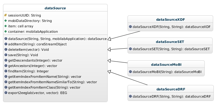
Figure 2: Data source hierarchy of classes.

dataSource

This is an abstract class that serves as a base for classes that implement interfaces between data acquisition systems or intermediate data formats and MoBILAB toolbox.

Properties

Property name	Type	Description
sessionUUID	string	Universal unique identifier that links all the data sets belonging to the same session. A session is defined as a raw file or collection of files recorded the same day and its derived processed files. To guarantee that files within the same session are traceable, the sessionUUID code is attached at the end of each file name. Example: dataset_1 : filename_1_sessionUUID.hdr, filename_1_sessionUUID.bin dataset_2 : filename_2_sessionUUID.hdr, filename_2_sessionUUID.bin dataset_n : filename_n_sessionUUID.hdr, filename_n_sessionUUID.bin
mobiDataDirectory	string	Path to the directory where the collection of files of one session are stored.
item	cell array	Cell array (list) of objects (handles), where each object represents one single data set. The objects connect to binary and header files in the mobiDataDirectory and come up to live as functional entities that "know" what to do with the data sets they handle.
container	mobilabApplication	The term container is used to refer to an object that can perform certain operations on the contained object but not the other way around. In this case, for a dataSource object the container is an object from the class mobilabApplication. The role of mobilabApplication is controlling the GUI, but because GUI needs change rapidly, a different class can be implemented to satisfy the new requirements in the front-end and still serve as container to the dataSource. This is a way of separating GUI programming from the rest of the application that may be more stable.

Methods

Method name	Description	Input arguments	Output arguments	Usage
dataSource	Creates a dataSource object. As this is an abstract class it cannot be instantiated on its own. Therefore, this constructor must be call only within a child class constructor.	mobiDataDirectory: Path to the directory where the collection of files are or will be stored. sessionUUID: String specifying the universal unique identifier common to all the files of the same session. container: This is usually a mobilabApplication object that connects the GUI with the low-level functions that each item in the data source may implement.	dataSource (handle)	obj@dataSource( mobiDataDirectory, sessionUUID, mobilab);
export2eeglab	Export an EEG structure combining multiple streams and event markers. This method takes care of aligning and re-sampling objects with different sampling rates. The first argument is a vector with the indices of the objects whose data will be concatenated (by the channel dimension) one after the other to make EEG.data. The second argument is a vector with the indices of the objects whose event markers will be used to populate EEG.event.	indicesData: Indices of objects whose channels will be concatenated and used to form EEG.data. indicesMarkers: Indices of objects whose event markers will be used to populate EEG.event. container: This is usually a mobilabApplication object that connects the GUI with the low-level functions that each item in the data source may implement.	EEG (EEGLAB structure)	% index_eeg_object: index of the object containing EEG data % index_marker_object: index of the object containing the event markers EEG = mobilab.allStreams.export2eeglab( index_eeg_object, index_marker_object);

Go to MoBILAB classes

dataSourceXDF

This class imports into MoBILAB files recorder by the Lab Streaming Layer (LSL) library saved in xdf or xdfz format.

Methods

Method name	Description	Input arguments	Output arguments	Usage
dataSourceXDF	Creates a dataSourceXDF object.	file: xdf or xdfz file recorded by LSL mobiDataDirectory: path to the directory where the collection of files will be stored	obj: dataSource object (handle)	% file: xdf or xdfz file recorded by LSL % mobiDataDirectory: path to the directory where the % collection of files are or will be stored. obj = dataSourceXDF( file, mobiDataDirectory );

Go to MoBILAB classes

dataSourceSET

This class imports EEGLAB .set files into MoBILAB. If the .set file contains an ICA decomposition it creates two objects, one for EEG and the other one (a child of the former) for the ICA data.

Methods

Method name	Description	Input arguments	Output arguments	Usage
dataSourceSET	Creates a dataSourceSET object.	file: EEGLAB set file mobiDataDirectory: path to the directory where the collection of files will be stored	obj: dataSource object (handle)	% file: EEGLAB .set file % mobiDataDirectory: path to the directory where the % collection of files are or will be stored. obj = dataSourceSET( file, mobiDataDirectory);

Go to MoBILAB classes

dataSourceMoBI

This class reads into MoBILAB the content of a folder containing MoBILAB files.

Methods

Method name	Description	Input arguments	Output arguments	Usage
dataSourceMoBI	Creates a dataSourceMoBI object.	folder: folder containing MoBILAB files	obj: dataSource object (handle)	% folder: folder containing MoBILAB files obj = dataSourceMoBI( folder );

Go to MoBILAB classes

dataSourceDRF

This class imports into MoBILAB files recorder by Datariver saved in drf format.

Methods

Method name	Description	Input arguments	Output arguments	Usage
dataSourceDRF	Creates a dataSourceDRF object.	file: drf file recorded by Datariver mobiDataDirectory: path to the directory where the collection of files will be stored	obj: dataSource object (handle)	% file: drf file recorded by Datariver % mobiDataDirectory: path to the directory where the % collection of files are or will be stored. obj = dataSourceDRF( file, mobiDataDirectory );

Go to MoBILAB classes

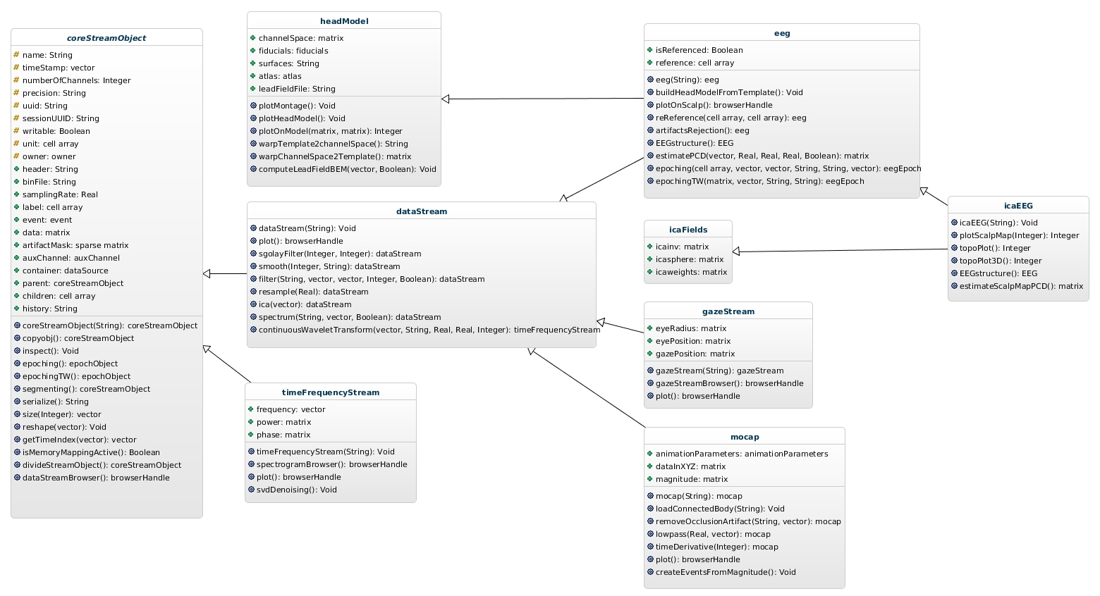
Figure 3: Data stream hierarchy of classes.

coreStreamObject

The class coreStreamObject serves as base to all stream objects.

Properties

"Property name	Type	Description
name	string	Name of the object. It usually reflects the operation that has created the object.
timeStamp	vector of doubles	Array of numbers containing the time stamps of each sample in seconds.
numberOfChannels	integer	Number of channels.
precision	string	Data precision.
uuid	string	Universal unique identifier. Each object has its own uuid.
sessionUUID	string	UUID common to all the objects belonging to the same session. A session is defined as a raw file or collection of files recorded the same day and its derived processed objects.
writable	logical	If true the object can be modified and even deleted, otherwise is considered raw data and it cannot be modified.
unit	cell array	Cell array of strings specifying the unit of each channel.
owner	struct	Contact information of the person who has generated/recorded the data set. It has the fields username, email, and organization. Even when supplying this information is optional it is highly recommended to do so. This info will keep other users from modifying a data set created by somebody else, for instance objects can be deleted only by its owner.
header	string	Pointer to the file containing the metadata, it has the following structure:path + object name + _ uuid _ sessionUUID .hdr
binFile	string	Pointer to the file containing the data that is going to be memory mapped. It has the following structure:path + object name + _ uuid _ sessionUUID .bin
samplingRate	double	Sampling rate in hertz.
label	cell array	Cell array of strings specifying the label of each channel.
event	event	Event object that contain event markers relative to the time base of the object that serves as container.
data	matrix	Matrix size number of samples (same as time stamps) by numberOfChannels. Data is a dependent property that access the time series stored in a binary file through a memory mapping file object. This makes possible working with data sets of any size, even if they don't fit in memory.
artifactMask	sparse matrix	Sparse matrix with the same dimensions of "data". Non-zero entries contain a number between 0 and 1 with the probability of the correspondent sample to be an artifact.
auxChannel	structure	Auxiliary channels whose type may be not the same as the data contained in obj.data. For instance a Trigger channel will go here. auxChannel.data contains the data and auxChannel.label the channel labels.
container	dataSource	Pointer to the dataSource object.
pointer	coreStreamObject	Pointer to the parent object. Object containing raw data have no parent, in this case it returns empty.
children	cell array	Cell array containing immediate descendant objects.
history	string	Command who has created the object. Calling this command will produce exactly the same data set. This field is very useful for the creation of scripts.

Methods

Method name	Description	Input arguments	Output arguments	Usage
coreStreamObject	Creates a coreStreamObject. As this is an abstract class it cannot be instantiated on its own. Therefore, this constructor must be called only from within a child class constructor.	header: header file (string)	obj: coreStreamObject (handle)	% executed from within a derived class constructor obj@coreStreamObject(header);
copyobj	Creates a new object calling the appropriated constructor.	parentCommand: structure with the following fields: 1) commandName (string), 2) uuid(string), uuid of the parent object, and 3) varargin, cell array of input arguments.	cobj: handle tho the new object	% eegObj is raw data it cannot be modified, if you need to % modify raw data in your own routines you can make a copy of it eegObj = mobilab.allStreams.item{ eegItem }; eegObj2 = copyobj( eegObj );
inspect	Pops up a figure showing all the published properties of the object.	None	None	% eegItem: index of some object containing EEG data eegObj = mobilab.allStreams.item{ eegItem }; eegObj.inspect; % observe that the following syntax is also valid inspect( eegObj ); The code above will produce a figure that look like this:
segmenting	Creates a new object containing only the data contained in the specified segments. Between every two segments a boundary event is inserted.	startEventMarkers: string or cell array of strings with the event marker signalizing the start of the segment endEventMarkers: string or cell array of strings with the event markers signalizing the end of the segment segmentName: string to be added to the name of the new object (optional), default "seg" channels: indices of the channels to include in the segmented object, default: all	segObj: segmented object	% eegItem: index of some object containing EEG data % event marker '701' -> Go % event marker '702' -> Stop eegObj = mobilab.allStreams.item{ eegItem }; segObj = eegObj.segmenting({'701'},{'702'}, 'walking');
serialize	Returns a serialized version of the object in a form of a JSON string.	None	JSON string	obj.serialize
size	Returns the two-element row vector containing the number of rows and columns in obj.data, where prod(size(obj.data)) is equal to length(obj.timeStamp) * obj.numberOfChannels. In case of reshaping the data size will return a vector with many elements as new dimensions.	dim: dimension, make size returns the length of the specified dimension	dimVector: vector with the length of each dimension of the data	eegObj = mobilab.allStreams.item{ eegItem }; dim = size( eegObj ); % number of time points , number of channels dim = size( eegObj, 1); % number of time points
reshape	Reshape obj.data.	dim: vector with the length of each new dimension	None	% mocapItem: index of some object containing mocap data mocapObj = mobilab.allStreams.item{ mocapItem }; dim = size( mocapObj ); reshape( mocapObj, [dim(1), 3 dim(2)/3]); figure; plot( mocapObj.timeStamp, mocapObj.data(:,1,1)); xlabel('Time (sec)'); title('X-coordinate of Marker 1');
getTimeIndex	Returns the indices correspondent to the input vector of time stamps.	latencyInSeconds: vector of time stamps in seconds	latencyInSamples: latency in samples.	eegObj = mobilab.allStreams.item{ eegItem }; latencyInSeconds = eegObj.timeStamp( 1: eegObj.samplingRate ); latencyInSamples = eegObj.getTimeIndex( latencyInSeconds ); samples = eegObj.data( latencyInSamples, :); figure;plot(latencyInSeconds, saamples); xlabel('Time (sec)'); title('First second of data');
isMemoryMappingActive	Returns true if the connection with the binary file is valid, otherwise returns false.	None	None	if isMemoryMappingActive(obj), disp('It is active.');end
divideStreamObject	Creates a new object from a subset of channels in the parent object.	channels : channels to keep labels : labels of the channels in the new object, if passed empty uses the labels in the parent object that correspond to the selected channels name: name of the new object, default: 'subSet_' + obj.name	cobj: handle to the new object	% Suppose we have used an EEG device with 128 channels, where the two groups % of consecutive 64 channels correspond to participants 1 and 2. This example % separates the data in one object per subject. eegObj = mobilab.allStreams.item{ eegItem }; % data subject 1 and 2 channels_1 = [1:64]; % channels subject 1 channels_2 = [65:128]; % channels subject 2 labels_1 = eegObj.label( channels_1 ); labels_2 = eegObj.label( channels_2 ); objectName_1 = [eegObj.name '_1']; objectName_2 = [eegObj.name '_2']; eegObj_1 = eegObj.divideStreamObject( channels_1, labels_1, objectName_1); eegObj_2 = eegObj.divideStreamObject( channels_2, labels_2, objectName_2);
dataStreamBrowser	Pops up a time series browser.	None	None	eegObj = mobilab.allStreams.item{ eegItem }; eegObj.dataStreamBrowser; The code above will produce a figure that look like this:

Go to MoBILAB classes

dataStream

This class serves as base class to all objects that representing some modality of time series data. It defines methods for re-sampling, smoothing, filtering, plotting, fft, and time frequency analysis.

Methods

Method name	Description	Input arguments	Output arguments	Usage
dataStream	Creates a dataStream object.	header: header file (string)	obj: dataStream object (handle)	obj = dataStream(header);
plot	Plots the time series in a browser window using the method dataStreamBrowser.	None	hBrowser: handle to the browser	eegObj = mobilab.allStreams.item{ eegItem }; plot( eegObj); % hBrowser = plot( eegObj); The code above will produce a figure that look like this:
sgolayFilter	Implements and applies a Savitzky-Golay filter. Savitzky-Golay smoothing filters (also called digital smoothing polynomial filters or least-squares smoothing filters) are typically used to "smooth out" a noisy signal whose frequency span (without noise) is large. In this type of application, Savitzky-Golay smoothing filters perform much better than standard averaging FIR filters, which tend to filter out a significant portion of the signal's high frequency content along with the noise. Although Savitzky-Golay filters are more effective at preserving the pertinent high frequency components of the signal, they are less successful than standard averaging FIR filters at rejecting noise. Savitzky-Golay filters are optimal in the sense that they minimize the least-squares error in fitting a polynomial to frames of noisy data.	order: order of the polynomial movingWindow: number of samples used in the least-square fitting of the polinomial. The size of the window must be odd, if order = movinWindow - 1. the filter produce no smoothing.	cobj: handle to the new object	order = 4; movingWindow = 33; obj = mobilab.allStreams.item{ itemIndex }; cobj = obj.sgolayFilter( order, movinWindow ); figure;plot( obj.timeStamp, [obj.data(:,1) cobj.data(:,1)] ); xlabel('Time (sec)'); legend({obj.name cobj.name});
smooth	Smooth the data.	movingWindow: length of the smoothing window (integer), default: 16 method: method of smoothing, can be moving, lowess, loess, sgolay, rlowess, rloess; default: moving channels: channels to smooth, default: all	cobj: handle to the new object	movingWindow = 32; method = 'moving'; obj = mobilab.allStreams.item{ itemIndex }; cobj = obj.smooth( movingWindow, method ); figure;plot( obj.timeStamp, [obj.data(:,1) cobj.data(:,1)] ); xlabel('Time (sec)'); legend({obj.name cobj.name});
firDesign	Designs a windowed linear-phase FIR filter using a Hann (Hanning) window. It calls internally the function fir1.	filterOrder: integer representing the order of the filter filterType: could be: 1) 'lowpass', 2) highpass, 3) 'bandpass', or 4) 'stopband' cutoff: vector of cutoff frequencies (in Hz) plotFlag: logical that if true plots the frequency response of the filter	b: coefficients of the filter	eegObj = mobilab.allStreams.item{ eegItem }; filterOrder = round(eegObj.samplingRate*1.25); cutoff = [1 128]; % assuming the sampling rate is > 256 Hz b = eegObj.firDesign( filterOrder, 'bandpass', cutoff, true); This code will produce the following figure:
filter	Design/applies or applies a zero-lag FIR filter.	Variant 1: filterType: can be: 1) lowpass, 2) bandpass, 3) highpass, or 4) bandstop cutoff: vector of cutoff frequencies (in Hz) channels: channels to filter, default: all order: order of the filter, default: 1024 plotFreqz: if true plots the frequency response of the filter Variant 2 b: filter's numerator's coefficients a: filter's denominator's coefficients	cobj: handle to the new object	eegObj = mobilab.allStreams.item{ eegItem }; % % Variant 1: eegObjFilt1 = eegObj.filter( 'bandpass', [1 45] ); % % Variant 2: % compute the coefficient of the filter by other method b = eegObj.firDesign( 640, 'bandpass', [1 45] ); eegObjFilt2 = eegObj.filter( b, 1 ); figure;plot( eegObj.timeStamp, [eegObj.data(:,1) eegObjFilt1.data(:,1)] ); xlabel('Time (sec)'); legend({eegObj.name eegObjFilt1.name}); figure;plot( eegObj.timeStamp, eegObjFilt1.data(:,1)-eegObjFilt2.data(:,1) ); xlabel('Time (sec)');ylabel('Variant1 - Variant2')
resample	Re-sample the time series. This method is implemented in two steps: 1) interpolation to match the new sampling rate and 2) in case of downsample it goes on to lowpass the signal to eliminate possible aliasing. You can change the sampling rate of the time series simply by changing obj.samplingRate. The set method of this property will call resample to do the job.	newSamplingRate: neew sampling rate	cobj: handle to the new object	eegObj = mobilab.allStreams.item{ eegItem }; % downsampling eegObj1 = eegObj.resample( eegObj.samplingRate/2 ); % upsampling eegObj2 = eegObj.resample( eegObj.samplingRate*2 ); figure; hold on; grid on; plot( eegObj.timeStamp, eegObj.data(:,1)); plot(eegObj1.timeStamp, eegObj1.data(:,1), 'g'); plot(eegObj2.timeStamp, eegObj2.data(:,1), 'r'); xlabel('Time (sec)'); legend({eegObj.name, 'donwsampled' 'upsampled'}); % without creating new objects you can simply run this: % eegObj.samplingRate = eegObj.samplingRate/2; % downsample % eegObj.samplingRate = eegObj.samplingRate*2; % upsample back to the original sampling rate This code should produce something like this:
ica	Performs the Independent Component Analysis of the time series. If a NVIDIA GPU card is available it uses cudaica (20x faster), otherwise uses binica. In both cases the InfoMax criteria is implemented. The method takes care of rank deficient data.	channels: channels to do ica on, default: all	cobj: handle to the new object	eegObj = mobilab.allStreams.item{ eegItem }; channels = 1:eegObj.numberOfChannels; icaObj = eegObj.ica( channels ); plot(icaObj);
spectrum	Computes the power spectral density (psd).	method: can be mtm (Thomson multitaper method), welch, periodogram, or yulear (Yule-Walker's method) channels: channels to compute the psd on, default: all plotFlag: if true plots the psd, default: true plotType: 2 or 3D plot, default: 2D	psdData: power spectral density (matrix) frequency: frequency axis (hertz)	eegObj = mobilab.allStreams.item{ eegItem }; method = 'welch'; channels = 1:10; plotFlag = true; [psdData,frequency] = spectrum( eegObj, method, channels, plotFlag); The PSD of EEG data could look like this: Observe that this an EEG that has been bandpassed between 1 and 128 Hz, it contains line noise (the peak at 60 Hz) and possible leaks from EMG, eye movements, etc.
continuousWaveletTransform	Computes the time-frequency representation of the time series using the Continuous Wavelet Transform.	channels: channels to compute the time frequecy decomposition of, default: all wavelet: name of the wavelet, could be: cmor1-1.5, morl, morlex, morl0, mexh, or paul fmin: minimum frequency in the frequency axis, default: 2 Hz fmax: maximum frequency in the frequency axis, default: obj.samplingRate/2 numFreq: number of frequencies, default: 64	cobj: handle to the new object	eegObj = mobilab.allStreams.item{ eegItem }; channels = 1:eegObj.numberOfChannels; wavelet = 'cmor1-1.5'; fmin = 2; fmax = 45; numFreq = 64; tfObj = eegObj.continuousWaveletTransform( channels, wavelet, fmin, fmax, numFreq); plot( tfObj );

Go to MoBILAB classes

eeg

The class eeg defines analysis methods exclusively for EEG data. It inherits signal processing methods from dataStream and incorporates routines for custom artifact rejection, filtering, and source localization. It also inherits from headModel fields and methods for co-registration of head shape and sensor coordinates, anatomic labeling of the cortical surface, and fast computation of the lead field matrix of realistic geometries by means of OpenMEEG.

Properties

Property name	Type	Description
channelSpace	number of sensors by 3 matrix	xyz coordinates of the sensors. Inherited from headModel.
fiducials	structure	xyz of the fiducial landmarks: nassion, lpa, rpa, vertex, and inion. Inherited from headModel.
surfaces	string	Pointer to the file where the surfaces representing different layers of tissue are stored. The surfaces must be in an array of MATLAB patches in the following order: 1) scalp, 2) skull, 3) brain (gray matter or average between gray and white matter). Inherited from headModel.
atlas	structure	Atlas correspondent to the most internal of the surfaces (gray matter). Inherited from headModel.
leadFieldFile	string	Pointer to the file where the lead field matrix was stored. Inherited from headModel.
isReferenced	logical	It reflects whether an EEG data set has been re-referenced of not.
reference	cell array	Labels of the channels used to compute the reference.

Methods

style="width: 15%; | Method name	Description	Input arguments	Output arguments	Usage
readMontage	Reads a file containing the sensor positions and its labels. If recorder, it also extracts fiducial landmarks. If the number of channels in the file are less than the number of channels in the object, a new object is created with the common set. If more than one file is supplied the program creates separate objects containing the different set of channels selected by each file.	file: filename. The following formats are supported: BESA or EGI3D cartesian .sfp, Polhemus .elp, Matlab .xyz or .sph, EEGLAB .loc, and Neuroscan .asc or .dat.	None	eegObj = mobilab.allStreams.item{ eegItem }; file = 'sensor_positions.sfp' eegObj.readMontage( file );
buildHeadModelFromTemplate	Builds an individualized head model that matches the channel space (sensor positions) of the subject. This methodology represents an alternative to cases where the MRI of the subject is not available. If no arguments are passed the program uses a default head model specified in mobilab.preferences.eeg.headModel	templateHeadModelFile: pointer to the template head model showModel: if true a figure with the resulting individualized head model is showed.	None	templateHeadModelFile = mobilab.preferences.eeg.headModel showModel = true eegObj = mobilab.allStreams.item{ eegItem }; eegObj.buildHeadModelFromTemplate( templateHeadModelFile, showModel); For plotting the resulting head model it uses the method plotHeadModel, explained below in this table.
plotMontage	Plots a figure with the xyz distribution of sensors, fiducial landmarks, and coordinate axes.	None	hFigure: handle to the figure	eegObj = mobilab.allStreams.item{ eegItem }; hFigure = plotMontage( eegObj ); This code should produce a figure like this:
plotHeadModel	Plots the different layers of tissue, the sensor positions, and their labels. It colors different regions of the cortical surface according to a defined anatomical atlas. Several interactive options for customizing the figure are available.	None	hFigure: handle to the figure	eegObj = mobilab.allStreams.item{ eegItem }; hFigure = plotHeadModel( eegObj ); The head model will look like this:
artifactsRejection	Automatic artifact rejection routines developed by Christian Kothe. It is highly recommended to run this pipeline before running ICA. No segments will be removed from the resulting stream object, although hopeless segments will be marked as artifacts in the field artifactMask. The pipeline implements different cleaning strategies in the following order: 1- remove flat-line channels, can be skipped making ''flatline_crit = 'off' '' 2- high-pass filter the data, can be skipped making ''highpass = 'off' '' 3- remove hopeless channels, can be skipped making ''channel_crit,'off' '' 4- repair high amplitude short period bursts, can be skipped if ''burst_crit = 'off' '' 5- remove hopeless time windows, can be skipped if ''window_crit = 'off' '' 6- interpolate removed channels from its neighbors, can be skipped if interp_crit_channel = false.	channel_crit: Criterion for removing bad channels. This is a minimum correlation value that a given channel must have w.r.t. at least one other channel. Generally, a fraction of most correlated channels is excluded from this measure. A higher value makes the criterion more aggressive. Reasonable range: 0.45 (very lax) - 0.65 (quite aggressive). burst_crit: Criterion for projecting local bursts out of the data. This is the standard deviation from clean EEG at which a signal component would be considered a burst artifact. Generally a higher value makes the criterion less aggressive.Reasonable range: 2.5 (very aggressive) to 5 (very lax). One usually does not need to tune this parameter. window_crit: Criterion for removing bad time windows. This is a quantile of the per-window variance that should be considered for removal. Multiple channels need to be in that quantile for the window to be removed. Generally a higher value makes the criterion more aggressive. Reasonable range: 0.05 (very lax) to 0.15 (quite aggressive). highpass: Transition band for the initial high-pass filter in Hz. This is [transition-start, transition-end]. interp_crit_channel: If true, interpolates critical channels using local-linear spacial Gaussian kernel. It uses the coordinates of three neighbor sensors to reconstruct the signal of the hopeless channels. channel_crit_excluded: The fraction of excluded most correlated channels when computing the Channel criterion. This adds robustness against channels that are disconnected and record the same noise process. At most this fraction of all channels may be fully disconnected. Reasonable range: 0.1 (fairly lax) to 0.3 (very aggressive); note that increasing this value requires the ChannelCriterion to be relaxed to maintain the same overall amount of removed channels. channel_crit_maxbad_time: This is the maximum fraction of the data set during which a channel may be bad without being considered "bad". Generally a lower value makes the criterion more aggressive. Reasonable range: 0.15 (very aggressive) to 0.5 (very lax).'). burst_crit_refmaxbadchns: The maximum fraction of bad channels per time window of the data that is used as clean reference EEG for the burst criterion. Instead of a number one may also directly pass in a data set that contains clean reference data (for example a minute of resting EEG; this has to be done from the command line). Reasonable range: 0.05 (very aggressive) to 0.3 (quite lax). burst_crit_reftolerances: These are the power tolerances beyond which a channel in the clean reference data is considered "bad", in standard deviations relative to a robust EEG power distribution (lower and upper bound). window_crit_tolerances: These are the power tolerances beyond which a channel in the final output data is considered "bad", in standard deviations relative to a robust EEG power distribution (lower and upper bound). flatline_crit: Minimum standard-deviation that a channel must have to be considered valid.	cobj: handle to the new object	% Executes the artifact rejection pipeline using default parameters. eegObj = mobilab.allStreams.item{ eegItem }; artFreeObj = eegObj.artifactsRejection;
plotOnScalp	Plot EEG data on the surface of the scalp.	None	None	eegObj = mobilab.allStreams.item{ eegItem }; eegObj.plotOnScalp; This method will pop-up a browser window like this:
computeLeadFieldBEM	Solves the forward problem of the EEG using Boundary Element Method on a realistic geometry. It uses OpenMEEG toolbox [1]. The computed lead field matrix is stored as a file in the field leadFieldFile. References: [1] Gramfort, A., Papadopoulo, T., Olivi, E., & Clerc, M. (2010). OpenMEEG: opensource software for quasistatic bioelectromagnetics. Biomedical engineering online, 9, 45. doi:10.1186/1475-925X-9-45 [2] Valdés-Hernández, P.A., Von Ellenrieder, N., Ojeda-Gonzalez, A., Kochen, S., Alemán-Gómez, Y., Muravchik, C., & A Valdés-Sosa, P. (2009). Approximate average head models for EEG source imaging. Journal of Neuroscience Methods, 185(1), 125–132. [3] Wendel, K., Malmivuo, J., 2006. Correlation between live and post mortem skull conductivity measurements. Conf Proc IEEE Eng Med Biol Soc 1, 4285-4288. [4] Oostendorp, T.F., Delbeke, J., Stegeman, D.F., 2000. The conductivity of the human skull: Results of in vivo and in vitro measurements. Ieee Transactions on Biomedical Engineering 47, 1487-1492.	conductivity: conductivity of each layer of tissue, scalp - skull - brain, default: 0.33-0.022-0.33 S/m. See [2, 3, 4] for details. orientation: if true, computes the orientation free lead field matrix, otherwise constrains the dipoles to be normal to the cortical surface.	None	% This example assumes a head model has been constructed for eegObj % See buildHeadModelFromTemplate for details of how to construct the % head model from a template. eegObj = mobilab.allStreams.item{ eegItem }; conductivity = [0.33 0.022 0.33]; % conductivity: scalp - skull - brain orientation = true; % orientation free dipoles eegObj.computeLeadFieldBEM( conductivity, orientation);
estimatePCD	Computes the posterior distribution of the Primary Current Density (PCD) given a topographic voltage. Being J a vector of PCD at each cortical dipole (vertices in the cortical surface) and V the EEG signal in channel space (measured on the scalp), the program computes the posterior distribution of the parameters J given the data V solving two levels of inference: 1) optimization of parameters J, and 2) optimization of hyper-parameters α and β. Level of inference 1 is addressed maximizing the posterior probability of the parameters J given the data V and hyper-parameters α and β: $P(J|V,\alpha,\beta) = \frac{P(V|J,\alpha)P(J|\beta)}{P(V|\alpha,\beta)}$ where α and β represent the precision of the noise in the scalp and the cortex (inverse variances). In level 2 the posterior of the hyper-parameters given the data and parameters is maximized: P(α, β|V) ≈ P(V|α, β)P(α, β) See Trujillo-Barreto et. al. (2004) for details. If the PCD is estimated at a single time point (one topography), the resulting inverse solution is theoretically equivalent to the method sLORETA described in Pascual-Marqui (2002). However, if the PCD is estimated in a continuous manner, the program uses updates equations for the hyper-parameters α and β derived from solving level of inference 2 mentioned above. Therefore, it is possible to track source activity under changes in noise levels at scalp and/or cortical scales. This last feature makes it suitable for online applications or long-lasting experiments because it can deal with changes in the conductivity of the scalp due to, for instance, sweating, and/or non-stationary brain dynamics at different time scales. References: : Trujillo-barreto, N. J, Aubert-Vazquez, E., Valdes-Sosa, P. A. (2004). Bayesian model averaging in EEG/MEG imaging. System, 21, 1300 – 1319. doi:10.1016/j.neuroimage.2003.11.008 : Pascual-Marqui, R.D., 2002. Standardized low-resolution brain electromagnetic tomography (sLORETA): technical details. Methods Find. Exp. Clin. Pharmacol. 24 (Suppl D.), 5 –12.	latency: vector of latencies (in samples) specifying the topographic maps to invert. maxTol: maximum tolerance in the convergence error of the hyperparameters, default: 1e-3 maxIter: maximum number of iterations, default: 100 gridSize: size of the grid where search for the first hyperparameters, default: 100 verbose: if true outputs messages about the convergence of the estimation process, default: true	J: Primary Current Density matrix, size number of verices in the cortical surface by number of latencies cobj: if requested, an object is created to store the solution J roiObj: if requested, an object is created to store the solution J collapsed in anatomical regions defined by the atlas	eegObj = mobilab.allStreams.item{ eegItem }; latency = 1369809:1371345; % from 2675.5 sec to 2678.5 sec ( 3 seconds % in total = 1537 time points) J = eegObj.estimatePCD( latency ); % estimates the PCD (cortical maps) continuously % in 1537 samples V = eegObj.data( latency, :)'; % correspondent topographical maps The figure shows the topographic and estimated cortical PCD maps at selected latencies. All maps where computed using the code above. Observe how the center of the activity moves from the place where the Temporal, Angular and Supra-marginal Gyrus meet going up via the Parietal Inferior Gyrus, to Postcentral Precentral and Frontal areas.
plotOnModel	Plots cortical/topographical maps onto the cortical/scalp surface.	J: cortical map size number of vertices of the cortical surface by number of time points V: topographic map size number of vertices of the scalp surface by number of time points; if V is empty, a single color is used simulating the skin figureTitle: title of the figure (optional)	hFigure: handle to the figure	eegObj = mobilab.allStreams.item{ eegItem }; % as a continuation of the example above,we can use plotOnModel to visualize % cortical and topographical maps interactively in the same figure eegObj.plotOnModel( J, V); The figure will look like this:

Go to MoBILAB classes

The headModel class encapsulates common routines used for solving the forward and inverse problem of the EEG and it is now hosted in a separate repository.

https://github.com/sccn/mobilab/wiki/files/MotionTrackerCorrectionTool1.00.zip