library(tidyverse)
library(reshape2)
library(stringr)
library(lubridatae)
library(colorspace)
library(viridis)
library(hrbrthemes)
library(ggplot2)
#Reading in files
data = read.csv("Data/web_log_data.csv")
- Duplicated value or missing value eliminate
- Apply date format using lubridate
- Web log format check
#summary of the data
summary(data)
                   ip                      date_time
 msnbot.msn.com      : 314   03/May/2005:14:05:47:   5
 visp.inabox.net     : 194   22/May/2005:14:14:34:   4
 egspd42466.ask.com  :  93   22/May/2005:14:15:31:   4
 cpe-147-10-88-128.ql:  67   23/May/2005:17:18:46:   4
 cpe-144-131-212-106.:  63   23/May/2005:20:29:51:   4
 bri-pow-pr3.tpgi.com:  53   01/May/2005:11:36:13:   3
 (Other)             :5082   (Other)             :5842
                              request          step           session
 /                                : 821   Min.   : 1.000    Min.   :   1.0
 /favicon.ico                     : 554   1st Qu.: 1.000   1st Qu.: 569.0
 /robots.txt                      : 395   Median : 3.000   Median : 994.5
 /eaglefarm/javascript/menu.js    : 370   Mean   : 4.795   Mean   :1005.0
 /eaglefarm/pdf/Web_Price_List.pdf: 296   3rd Qu.: 6.000   3rd Qu.:1432.0
 /eaglefarm/                      : 286   Max.   :63.000   Max.   :1939.0
 (Other)                          :3144
    user_id
 Min.   :   1.0
 1st Qu.: 569.0
 Median : 994.5
 Mean   :1005.0
 3rd Qu.:1432.0
 Max.   :1939.0
We could expect the session and user_id are same column
## Find NA value
find_na = apply(is.na(data),2,sum)
print(find_na)
ip | date_time  | request |  step  | session  | user_id |
 0 |     0      |    0    |    0   |   0      |   0     |
Data columns have not missing values
#Identical Column check
print(identical(data$session , data$user_id))
[1] TRUE
It is found that session and user_id two columns are same. So I will delete 'session' column
#Apply Date Format. Use day, month, year, and hour
timeline = dmy_h(substr(data$date_time , 1, 14) )
# Request value check
print(unique(data$request)[40:55] )
[1] /code/Ultra/stationery.htm /code/Ultra/styling.css
 [3] /code/soon.html            /code/ultra/laminating.htm
 [5] /code/ultra/offset.htm     /code/ultra/photocopy.htm
 [7] /code/ultra/poster.htm     /code/ultra/stationery.htm
 [9] /direct                    /direct.html
[11] /eaglefarm                 /eaglefarm.html
[13] /eaglefarm/                /eaglefarm/aboutus
[15] /eaglefarm/aboutus/        /eaglefarm/contact
114 Levels: / ... /wynnum.html
We could find the Address /main and /main/ are treated different value. But it's same in web page. So I will eliminate last of '/'
## Eliminate last of '/'
lastChar_substr = function(x){
    lastChar = str_sub(x,-1)
    if(lastChar=="/" & str_length(x) >1){
        str_sub(x,-1) = ""
    }
    return (x)
}
data$request = sapply(as.character(data$request), lastChar_substr,USE.NAMES = FALSE)
Finally I will use data named 'data_timeline' to EDA
#Get preprcoessed data
data_timeline =  data %>%  mutate(timeline = timeline) %>% select(-c(date_time,session))
- I tried to visualze of Data and find meaningful insight.
## Period of Data
print(paste("Start Date :", min(data_timeline$timeline)))
print(paste("Last Date :", max(data_timeline$timeline)))
Start Date : 2005-04-18 21:00:00
Last Date : 2005-05-31 10:00:00
Data have values from 2015-04-18 to 2015-05-31 log
## User number analysis
session_n = data_timeline %>% group_by(user_id) %>% summarise(n=n())
print((paste("Total number of users :", nrow(session_n))))
Total number of users : 1939
## Visualize user number by total session
session_n %>%
    arrange(desc(n)) %>%
    ggplot(aes(n)) +
    geom_histogram(stat = "bin", binwidth=2 , fill = "#ffd62d" , col = "#ffd62d")+
    labs(title = "Number of User Count",x = "Total Session",y = "Count")+
    theme_ft_rc()+
    theme(plot.title = element_text(hjust = 0.5),legend.position = "None")
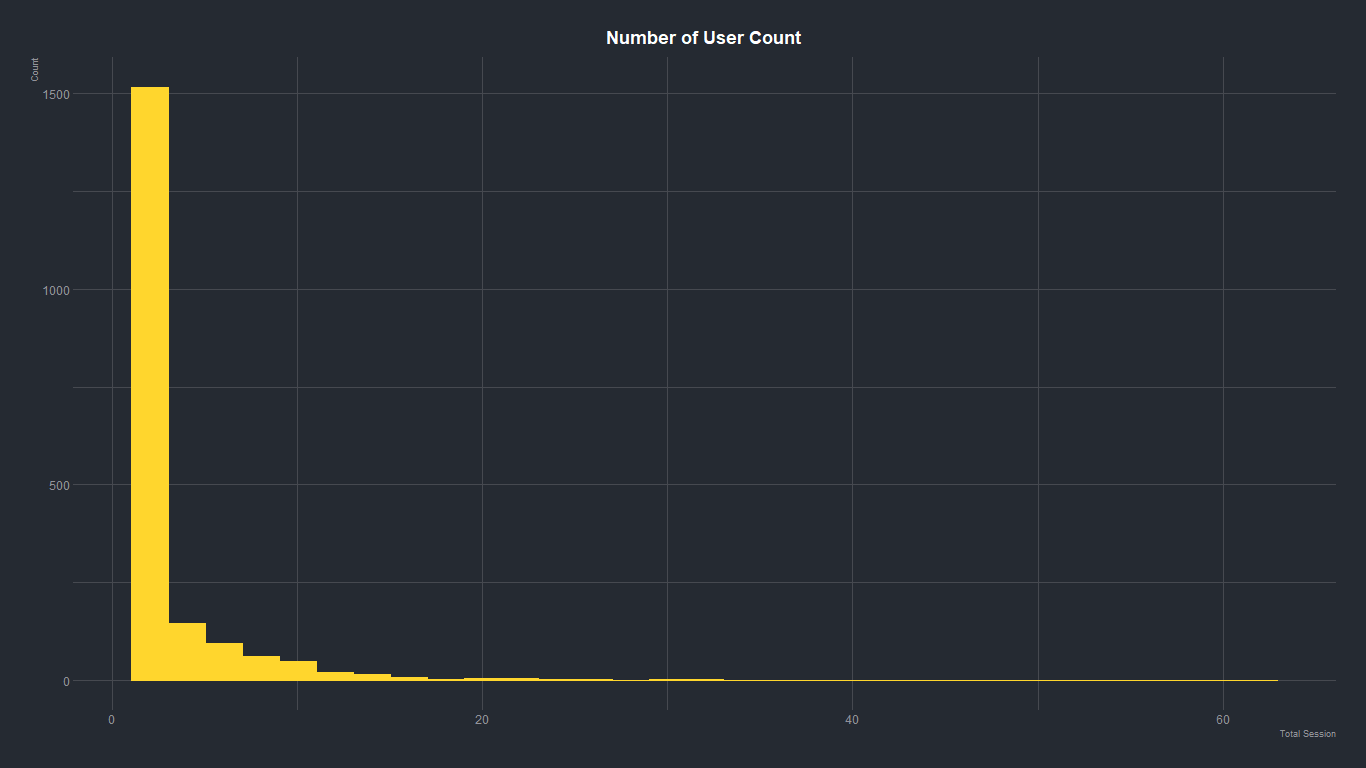 As above, Web user session number is skewed. And about half of users only have 1 session.
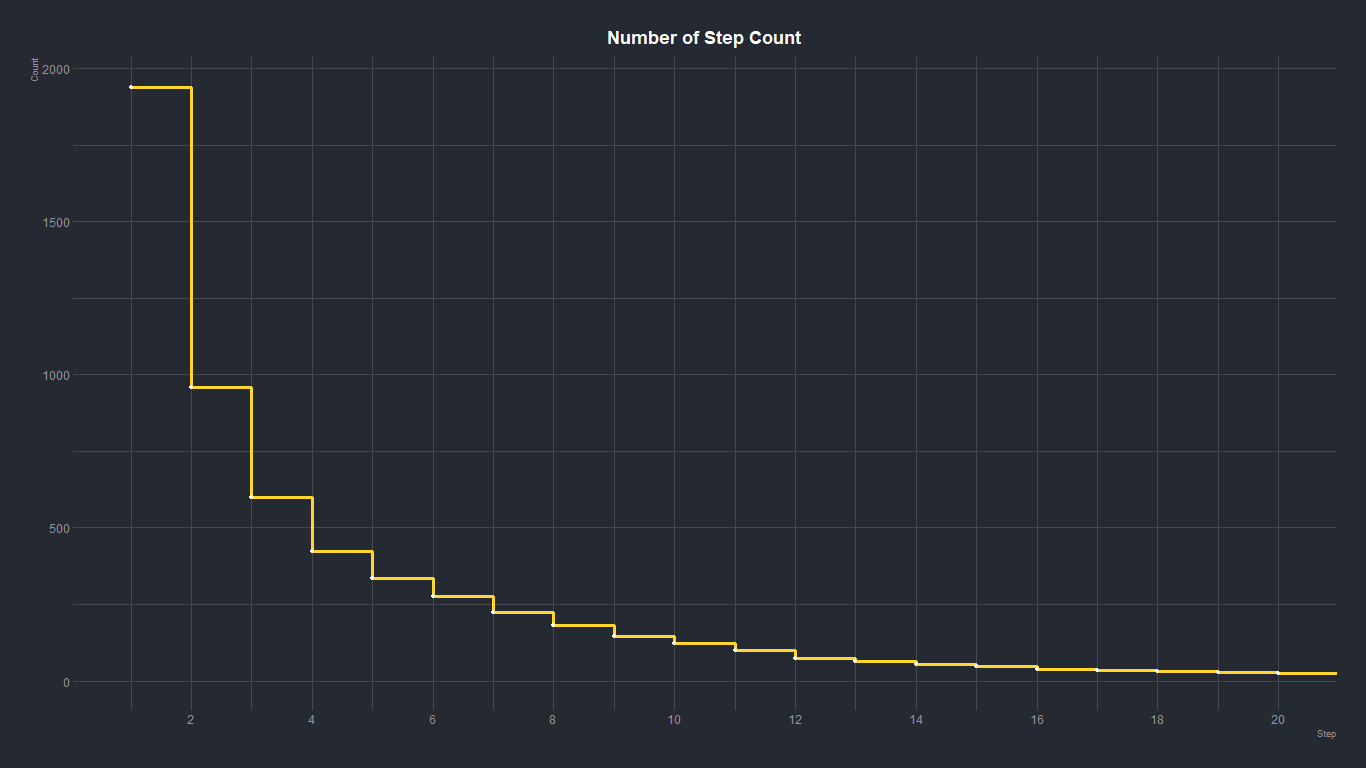
# Step number analysis
step_n <- data_timeline %>% group_by(step) %>% summarise(n=n())
## Visualize Step number
step_n %>%
    arrange(desc(n)) %>%
    ggplot(aes(x=step,y=n)) +
    geom_step(size=1.2, color="#ffd62d")+
    geom_point(size=1.5, color="#FFFFFF")+
    scale_x_continuous(breaks = scales::pretty_breaks(n = 10))+
    coord_cartesian(xlim = c(1, 20))+
    theme_ft_rc()+
    labs(title = "Number of Step Count",x = "Step",y = "Count")+
    theme(plot.title = element_text(hjust = 0.5),
          legend.position = "None")
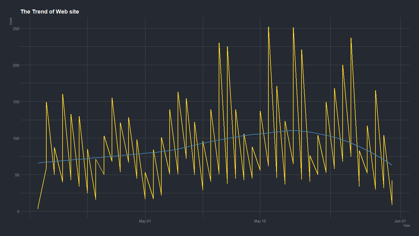
## Aggregated by Day
day_n <- data %>%
    group_by(day = floor_date(data_timeline$timeline, "day")) %>%
    summarise(n_person=n_distinct(user_id),n_session = n())
## Visualize trend of user and session by day
melt(day_n,id.var = "day")  %>%
    ggplot(aes(x=as.Date(day),y=value)) +
    geom_line(size=1,color="#ffd62d") +
    geom_smooth(method= 'loess',se = FALSE,color = "steelblue") +
    labs(title = "The Trend of Web site",x = "Date",y = "Count")+
    theme_ft_rc()
## Aggregated by hour
dat_hour <- data_timeline %>% group_by(hour = hour(timeline)) %>% summarise(n=n())
## Visualize hour distribution of Session
dat_hour %>%
    arrange(desc(n)) %>%
    ggplot(aes(x=hour,y=n,fill=cut(hour,4))) +
    geom_bar(stat="identity") +
    scale_fill_discrete_qualitative(palette = "Set 2")+
    theme_ft_rc() +
    labs(title = "The Hour Distribution of Session",x = "Hour",y = "Count")+
    theme(plot.title = element_text(hjust = 0.5),
          legend.position = "None")
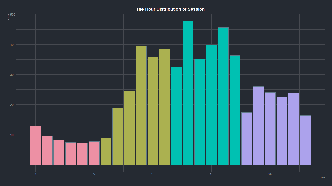 We could see the peak time of use is about 1 pm. and the use of web decrease after 6 pm.
## Aggregate dy IP
ip_n <- data_timeline %>% group_by(ip) %>% summarise(n=n())
top_n(ip_n, n=20, n) %>%
    arrange(desc(n)) %>%
    ggplot(aes(x=reorder(ip, n),y=n )) +
    geom_segment( aes(x=reorder(ip, n), xend=reorder(ip, n), y=0, yend=n), color="#fbde0e") +
    geom_point( color="#ffac2d", size=4) +
    coord_flip() +
    theme_ft_rc()+
    labs(title = "Number of IP Count",x = "IP",y = "Count")+
    theme(
        panel.grid.major.y = element_blank(),
        panel.border = element_blank(),
        axis.ticks.y = element_blank()
    )
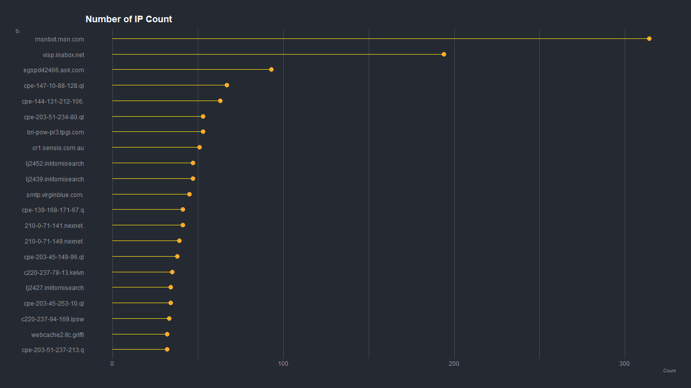 We could see IP of msnbot.msm.com and visp.inabox.net have large proportion. But I couldn't guess why that IP appear so many times.
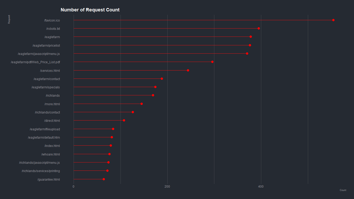
- Top 20 Request
##Aggregate by Request
request_n <- data_timeline %>% group_by(request) %>%
    filter(request!="/") %>% #exclude main page
    summarise(n=n())
# Horizontal version
top_n(request_n, n=20, n) %>%
    arrange(desc(n)) %>%
    ggplot(aes(x=reorder(request, n),y=n)) +
    geom_segment( aes(x=reorder(request, n), xend=reorder(request, n), y=0, yend=n), color="#fb0e0e") +
    geom_point( color="red", size=4) +
    labs(title = "Number of Request Count",x = "Request",y = "Count")+
    coord_flip() +
    theme_ft_rc()+
    theme(
        panel.grid.major.y = element_blank(),
        panel.border = element_blank(),
        axis.ticks.y = element_blank()
    )