Preparing climatic data for analysis with R Instat

1) Introduction

R-Instat is designed as a general statistics package. All the calculations are made through the statistical system called R. In addition, there is a special climatic menu.
In the future we plan for the climatic menu to facilitate the analysis of climatic data at any scale, e.g. from an automatic station. Currently the methods are particularly designed for daily data. This guide uses an example of daily data for 2 stations in Guinee (Conakry) each of which was supplied with 4 elements. These data are in the R-Instat library and hence the examples in this guide can be followed by users who wish to do so.

2) Acknowledgement

We gratefully acknowledge the permission of the Guinee Met Service for their permission to use their data in preparing this guide, and to allow their data to be added to the R-Instat library.

3) Getting the data into shape

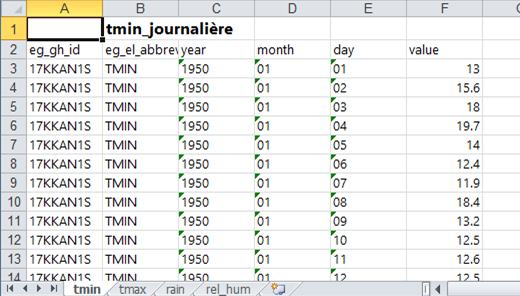
We first open the data in roughly the form it was originally presented. This is in 2 Excel files and hence we start by showing the data in Excel, rather than in R-Instat, Fig. 1.

Fig 1. The Data for one station in Excel	Fig 2. The shape used by R-Instat

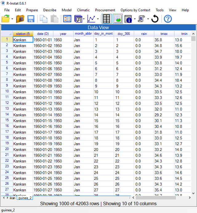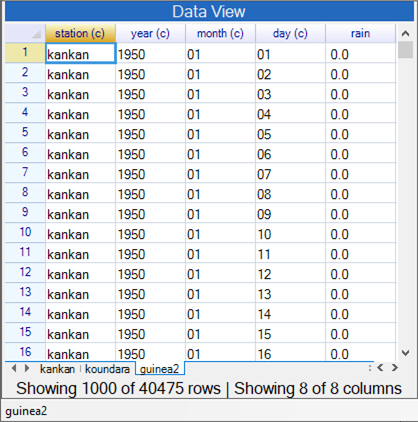
The data are in the right “shape” for R-Instat, i.e. one row of data for each day. The data for this station start in 1950 and continue to 2016 or 2017.
This is not always the case and in Appendix 1 we consider how to transform data that start in different “shapes”.
If your data are already in the right “shape”, as shown in Fig. 2 (and also Fig. 22) then you could jump to Section 4 of this guide. This shape has the 4 elements and both stations in the same data frame. The elements in Fig. 2 are in successive columns. The stations are one below the other, with the first column in Fig. 2 giving the station name.
There are also 4 sheets in the Excel file, Fig. 1, with a different element on each sheet. If the analysis is only for a single element, and for just this one station, then these data can be imported into R-Instat as shown below, and then continuing with Section 4. However, many analyses benefit from the data in these 4 sheets being merged into a single file. They can also be combined with those from the second station. That is what we show here.
Our aim is for the four elements, for both stations, to be in a single sheet or data frame.

• Go into R-Instat.
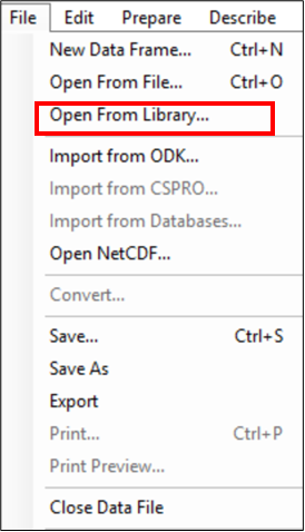
• Use File > Open from Library to open the data file, see Fig. 3.

(That is because these data are in the Instat library. For your own data use File > Open instead and look for the file.)

Fig 3. File > Open from library	Fig 4. Load from the Instat Collection

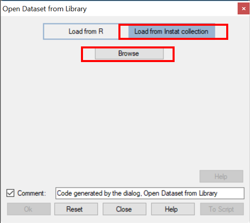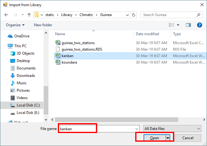
• Click on Load from Instat collection, Fig. 5.
• Click Browse, then choose Climatic and then Guinea.

Fig. 5 Choose the Excel file	Fig. 6 The resulting dialog

• Choose the file called kankan.xlsx and click on Open, Fig, 5.
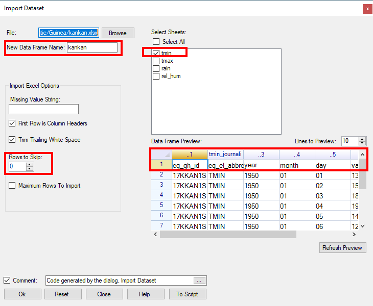
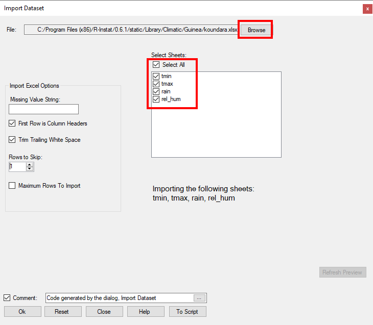
• Examine the dialogue, Fig. 6. Do NOT yet click OK. The current Excel sheet is not ready to import.
  One issue is clearer from another look at the data in Excel in Fig. 1. The first row is a heading, and the variable names are in row 2 of the sheet.
• Change the Rows to Skip to 1, because we can see in the Data Preview that we want to ignore the first row. Fig. 6.
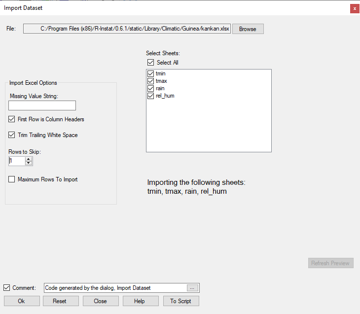
• Then click on the check boxes to select all four sheets which contain four elements. The results now look as in Fig. 7.

Fig. 7 The data ready to import	Fig. 8 Data in R-Instat

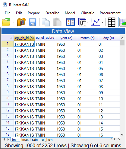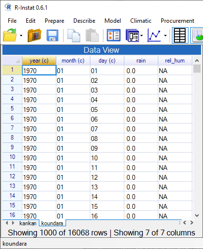
• Click OK to import the data into R-Instat, Fig. 8.

The bottom of Fig. 8 indicates there are 22,521 days, i.e. rows of data, of which only 1000 are shown. The grid in R-Instat is just a window showing part of the data. They are stored in R.
You now have 4 data frames in R-Instat shown on Fig 8. The tmax data frame has 22215 rows of data. There are 24080 rows of rainfall data and 11,045 rows for relative humidity.

Fig. 9 The Prepare Menu

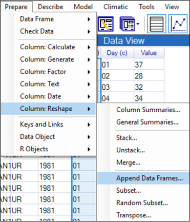The next task is to merge the data for the different elements into a single data frame. This is done in 2 stages. As we are preparing the data, this uses the Prepare menu, Fig. 9

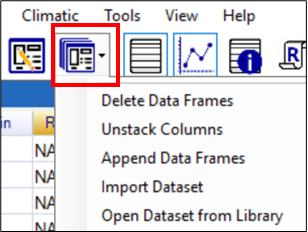
• In the Prepare menu, choose Data: Reshape and then Append Data Frames, Fig. 9.

Fig. 10 The Append dialog	Fig. 11 Append Completed

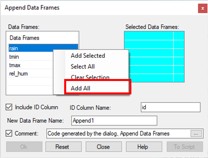
In the resulting dialogue you want to use all the data frames.

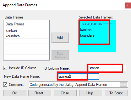
• Right-click in the data selector, see Fig. 10. Then choose Add All.
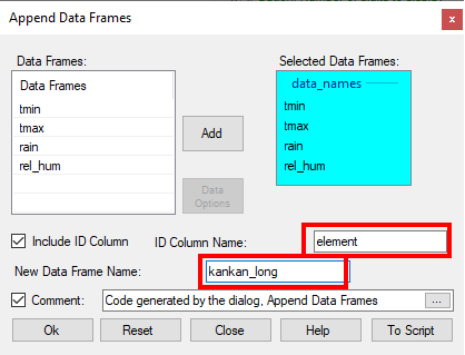
• Change the ID column name to element and the Data Frame name to kankan_long. Fig. 11.
• Press OK,
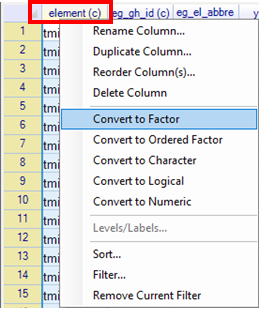
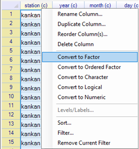
  This has produced a new data frame with 79,861 rows of data. The first column, called element is a text (character) type of column. It must be converted into a category type, which is called a Factor column in R.
• Right-click on the name element. This gives the pull-down menu shown in Fig. 12.
• Choose Convert to Factor. An (f) now appears after the column name.

Fig. 12 The right click menu	Fig. 13 Unstack

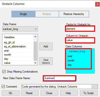• Use Prepare > Data: Reshape > Unstack, see Fig. 9 again.
  Complete the unstack dialogue as follows, see Fig. 13.
• The factor is the element column, while the Column to Unstack is value.
• There are 3 ID columns, namely year, month, day and the New Data Frame is called kankan.
• Press Ok.

Fig. 14 Right-click on the data frame	Fig. 15 The kankan data in the R-viewer

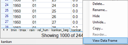
The grid, or spreadsheet, in R-Instat is just a window showing part of the data.

• Right-click on the name kankan, Fig. 14, and choose View Data Frame.
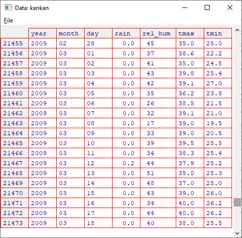
• Scroll down the data in the R-viewer, Fig. 15, to see the complete data.
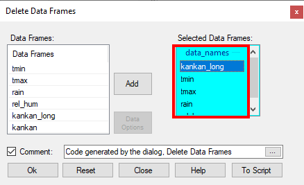
  Finally, for these data, we now delete the other data frames. The only one needed is kankan.
• Choose the kankan_long data frame.
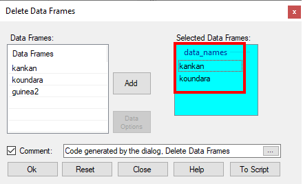
• Right-click at the bottom of the window, see Fig. 14 again, and choose Delete, Fig. 16.
• Add the other data frames – except kankan, of course - see Fig. 16!

Fig. 16 Deleting Unwanted data frames	Fig. 17 The recent dialogs used

• Press OK. The dialogues used so far are now also easily available, through the toolbar.
• Click on the icon, Fig. 18, to see what has been used.
• In the list – Fig. 17 – choose Import Dataset.
• In the resulting dialogue, Fig. 18, use Browse and choose the second station, koundara.

Fig. 18 A second data set	Fig. 19 Data from two stations

• Choose the file called koundara.xlsx and click on Open.
• Examine the dialogue, Fig. 18. Do NOT yet click OK. Click on the check boxes to select all four sheets which contain four elements. The results now look as in Fig. 18. The current Excel sheet is not ready to import.
• Now repeat the steps from Fig. 8, page 3, to Fig. 17, page 6, for the koundara data.
  The results, with the 2 data frames are in Fig. 19
• Use Prepare > Data: Reshape > Append again, see Fig 20 to put the data into a single data frame.

Fig. 20 Appending the data for the two stations	Fig. 21 Data for the two stations

This stage is now over. The data for both stations, and with all four elements, are in a single data frame, Fig. 21. There are 40475 rows (days) of data.
To complete the initial task the resulting files are now saved.

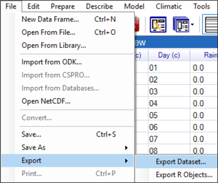
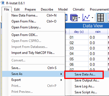
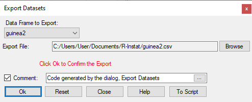
• Choose File > Export > Export Dataset, Fig. 22.

Fig. 22 Export and save the data	Fig. 23 Choose where to export the data

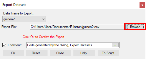• Click on Browse, Fig. 23, and choose where to save the exported file.
• After choosing the file name, you return to Fig. 23. Click OK. The file is not saved until OK is clicked
  By default, it is a csv file, which can easily be read into Excel.
• Right click on the kankan name at the bottom of the data frame.
• Select Delete, Fig. 24, to delete the individual station data.
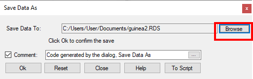
• Choose File > Save As > Save Data As, Fig. 25, to save a file of type RDS for reading back into R-Instat.

Fig. 24 Delete the extra data frames	Fig. 25 File > Save As

Review

This first stage has organised the data, ready for climatic analyses with R-Instat. The main task has been to reshape the data into the form used by R-Instat. The details of this stage depend on the original “shape” of the data. Other common starting points are considered in Appendix 1. We used the File menu and then the Prepare menu in R-Instat. Within the Prepare menu we particularly used the sub-menu Prepare > Data: Reshape and then used the Append and Unstack dialogues. Other data formats use additional options from this sub-menu, particularly Stack and Merge.

4) Adding a date column

• If you are continuing from the section above, that is fine. Continue with the data.
• (Otherwise start by loading the data you saved above. Or go again to File > Open from Library > Load from Instat Collection > Browse > Climatic > Guinea and choose the file called guinea_two_stations.csv.)

Fig. 1 Convert Station to a factor column	Fig. 2 Make Year, Month, Day Numeric

• Right-click on the station name and choose Convert to Factor, Fig. 1.
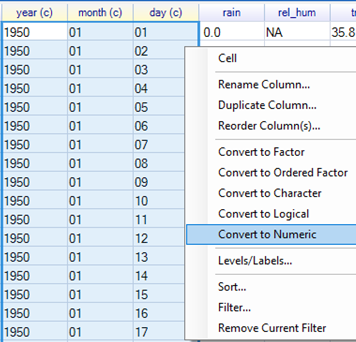
• Right-click also on the year, month and day columns (you can mark them all at once) and convert them to numeric, Fig. 2.

Now we check the data are roughly as they should be. Surprises are not wanted!

Fig. 3 Choose the Summarize dialog	Fig. 4 Right-click to choose all variables

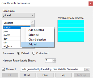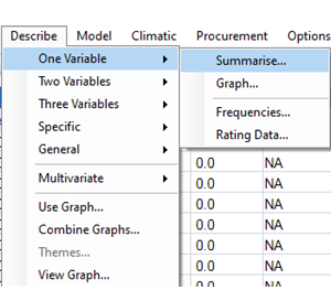
• Choose Describe > One Variable > Summarise, Fig. 3.

Notice, Ok is not enabled in the dialogue. It first needs some variables to summarise.

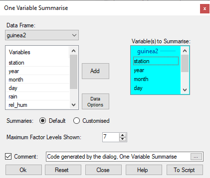
• Right-click in the data selector, Fig. 4, and choose the option to Add All. (Or just select all the variables and press the Add button.)

Fig. 5 Summarise dialog completed	Fig. 6 Results

The dialogue is now completed and hence the Ok button is enabled.

• Press Ok.
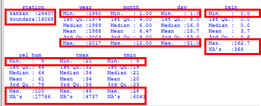
• Examine the results – some interesting points are marked in red in Fig. 6. They include:
  • The _station _ factor has just 2 levels. This is as expected, because we have 2 stations. There are more data for Kankan than Koundara and there are no missing values in this variable.
  • For the _rain _ column, the minimum is zero (dry day) and the maximum is 163mm. These are plausible values. There are less than 400 missing values. They are denoted by NA in R.
  • The year, month, day columns are also as expected, for example Day is between 1 and 31 and there are no missing values.
  • There are more missing values in the other 3 climatic elements. For these elements the minimum and maximum values are reasonable.
  • There are no really odd values, like -99 that should have been made into missing values. That’s all comforting.

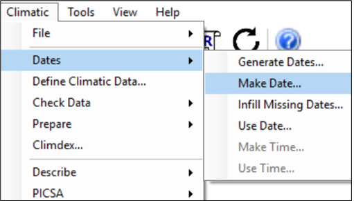
The next step is to make a single date variable.

• Choose Climatic > Dates > Make Date, Fig. 7.

Fig. 7 Add a date variable	Fig. 8 The Climatic > Date > Make Date dialogue

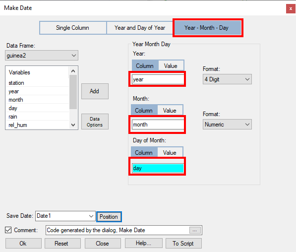• In the dialogue, Fig. 8 choose the Year – Month -Day button, because these 3 columns are in the current data frame.
• Complete the dialogue by **adding **the three columns, as shown in Fig. 8. Press Ok.

This has added a date column – of type (D) into the data frame.
The next step is to check whether any dates are missing from the file. This is not quite the same as missing values, but is when dates themselves are missing, perhaps whole years have been omitted from the file?

• Check the length of the data frame – currently 40475 rows (days) of data.
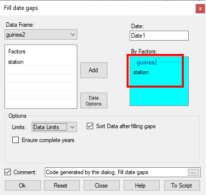
• Choose Climatic > Dates > Infill Missing Dates Fig. 9.

Fig. 9 Climatic >Dates > Infill	Fig. 10 Resetting one variable summarise

In Fig. 9 you should find the Date field was filled automatically.

• Click in the By Factors field and add the Station column, Fig. 9.
• Click Ok.

The length has now changed to 42063 rows. So about 1600 rows (days) have been added.

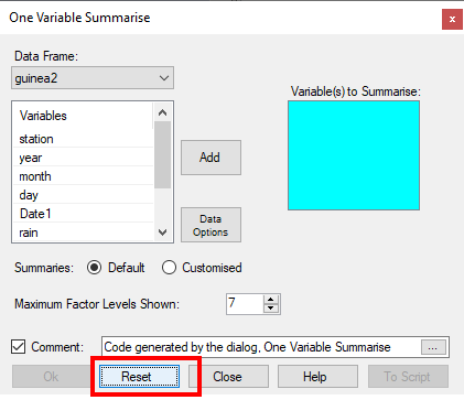
• Now use the Describe > One Variable > Summarise dialogue again. (Remember you also have a toolbar button to recall the last 10 dialogues.)
• Press the Reset button, Fig. 10.
• Right-click in the data selector (as you did before, Fig. 4) and Add All.
• Press Ok.

Fig. 11 Results from Describe > One Variable > Summarise

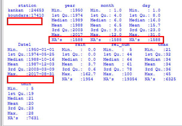The results are shown in Fig. 11. Because the data have been infilled, there are now missing values in the Year, Month and Day columns. Something must be done about this. Fortunately, there are no missing values in the Date and the Station columns.

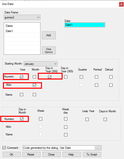
• Choose Climatic > Dates > Use Date, see Fig. 4 for the menu.
• Complete it as shown in Fig. 12.
• Press Ok.

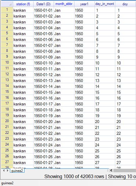
This has generated 4 new columns, Fig. 13, for the year, the month (with labels), the day in the month, and the day of the year. The first 3 can replace the original columns which now have missing values after the infilling.

Fig. 12 Climatic > Dates > Use Date	Fig. 13 Resulting columns generated

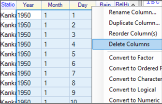
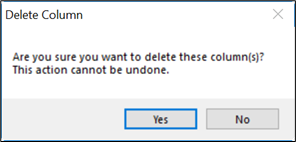
• Select the 3 original columns (now unwanted), right-click and choose Delete Columns, Fig 14.
• Confirm the deletion, Fig. 15.

Fig. 14 Delete unwanted columns	Fig. 15 Confirm the deletion

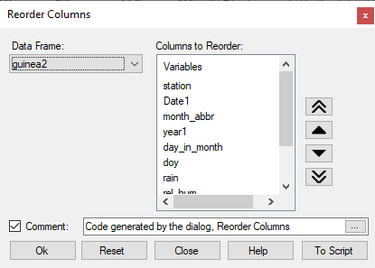
Finally, for this section, re-order the columns in the data frame, so the date columns are before the data.

• Right-click in the name field again, and choose Reorder Column(s), see Fig. 14.
• Reorder the columns as shown in Fig. 16.
• Press Ok. The data frame is now as shown in Fig. 17.

Fig. 16 Reorder columns in the data frame	Fig. 17 The resulting data

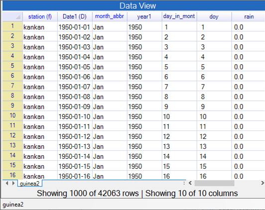You could now save the data as described earlier, see section 3. But the next section is very short and could perhaps be done first.

5) Define the data as climatic

The final preparatory stage is to define the data as climatic.

• Use Climatic > Define Climatic Data, Fig. 1.

Fig. 1 Climatic > Define Climatic Data

For this data set the dialogue was completed automatically. That is because R-Instat recognised the names of the columns. Otherwise the dialogue must be completed manually.

• Press Ok.

In the output window you see a summary of the data after being defined as climatic, Fig. 2.

Fig. 2 Defined Climatic Data	Fig. 3 The column metadata

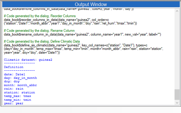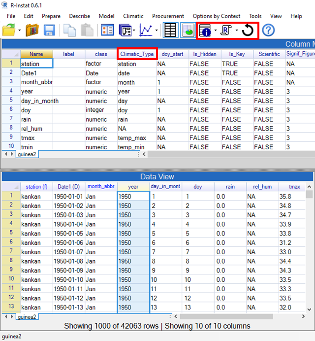This summary can also be viewed in another window in R-Instat. So, we take this opportunity to introduce a third window in R-Instat. So far you have seen a window for the data and another for the results.

• On the toolbar press the icon with an i – for information, Fig. 3.
• Drag to make this metadata window bigger, as shown in Fig. 3

This window has a row that corresponds to each column in the Data window. What is new after the dialogue in Fig. 1 is that the column metadata includes the Climatic_Type information.
This simplifies the dialogues for climatic analyses in further sections of this guide.
Notice also that a label can be added to give further details about the contents of any column.
** Press the i button on the toolbar again to close the metadata window. Alternatively use the curly arrow to reset the windows back to their default positions.

Finally, in this section, save the data. This is now ready to start the analyses.

• Use File > Save As > Save Data As to give the dialogue shown in Fig. 4.
• Click on Browse, Fig. 4 and choose where to save the data.

Fig. 4 File > Save As > Save Data As	Fig. 5 Exporting the data

• Click Save on the resulting dialogue, to return to Fig. 4.
• Click Ok which is the step that actually saves the file.
• If you wish, you can also choose File > Export > Export Dataset, Fig. 5. Then, click Browse, Save, and press Ok.

The export has saved a csv file. This can be viewed in Excel, and later imported back into R-Instat. However, it does not save the metadata.

6) Checking data quality

• Continue with the data file from the sections above.
• (Otherwise use File > Open from Library > Load from Instat Collection > Browse > Climatic > Guinea and open the file guinea2.RDS )

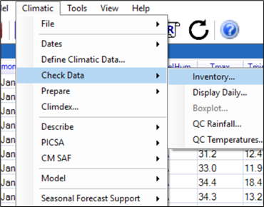
Fig. 1 Climatic menu	Fig. 2 Climatic > Check Data > Inventory

Section 4 showed menu options for the Dates and Section 5 used the Define Climatic Data dialogue. We now continue with dialogues that support checking the data.

• Choose Climatic > Check Data, Fig. 1.
• Choose the Inventory dialogue from the menu in Fig. 1.
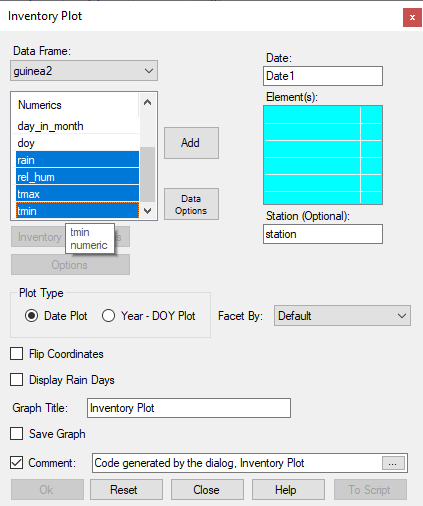
• In Fig. 2 Select the Elements receiver, then choose the 4 climatic elements and press Add.
• Press Ok.

Fig. 3 Inventory plot for Kankan and Koundara	Fig. 4 Dialogue for a second plot

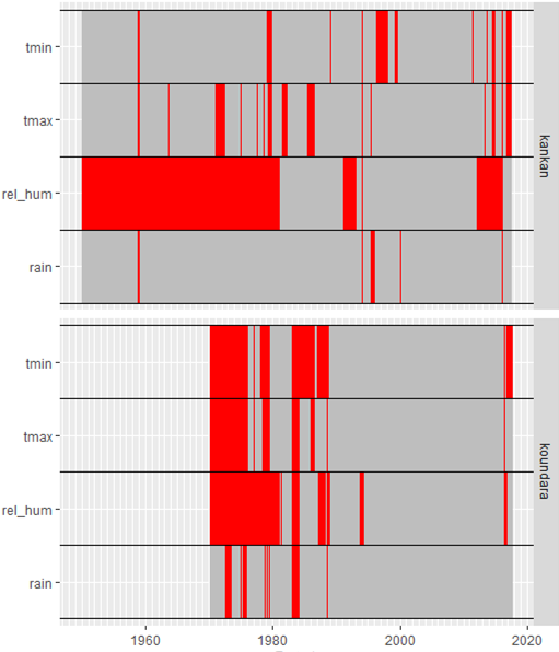
The top graph in Fig. 3 is for Kankan. The red indicates missing data and the record for the rainfall shows few missing values. The temperature data for Kankan also start in 1950. There are slightly more missing values, particularly for Tmax.
The rainfall data for Koundara start in about 1970, but the temperature data start a few years later. There are occasional missing periods in the early part of the rainfall record, but almost none later.

• Return to the Inventory dialogue. (Use the toolbar icon.)
• Press the Reset button, Fig. 4.
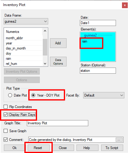
• Just put the rain variable into the receiver, Fig. 4.
• Set the other 2 options as shown in Fig. 4 to display the rain days, and to show days in the year.
• Press Ok to give the results in Fig. 5.

The results in Fig. 5 indicate a single rainy season at both sites, with a longer season at Kankan. The data give an overall impression of good quality, e.g. there are no very odd years in the record.

Fig. 5 Pattern for rainfall

The next option in Climatic > Check Data presents daily values in more detail.
This is slow for large amounts of data. We first filter to look just at the early years at Koundara.
Filtering is a powerful facility in R-Instat.

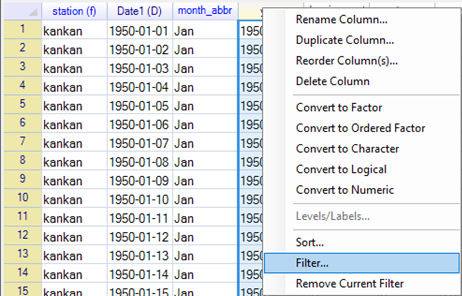
• Put the cursor in the name field of the data and right-click, Fig. 6.

Fig. 6 Selecting Filter	Fig. 7 Define a new filter

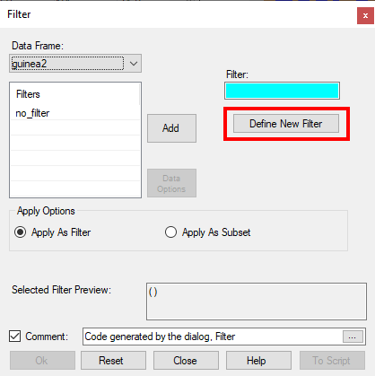• In the Filter dialogue, click to define a new filter, Fig. 7.

Fig. 8 Filter for level of a factor	Fig. 9 Filter for particular years

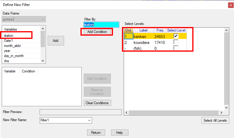
First select the station.

• Choose to filter on the Station variable, Fig. 8..
• Choose Koundara, rather than Kankan, Fig. 8. Then click to Add Condition.

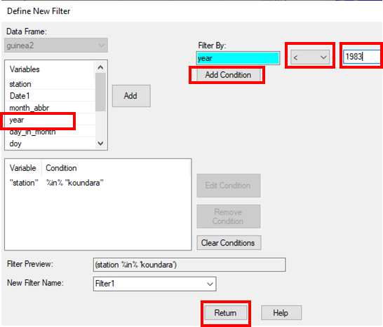
In Fig. 9, notice that the Station condition has now been added -It says “Station %in% 'Koundara'”. Now we add a further condition as well.

• Choose the year column, Fig. 9.
• Set the condition to < and type the year as 1983, Fig. 9.
• Click to Add Condition
• Now that the 2 conditions are added, press Return.

Fig. 10 The filter has been defined	Fig. 11 The filter is applied

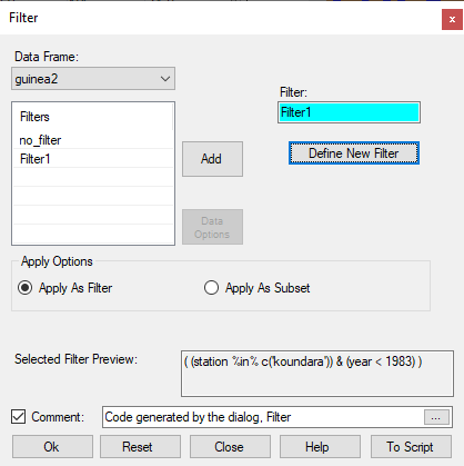
• Back on the main Filter dialogue, Fig. 10, press Ok.

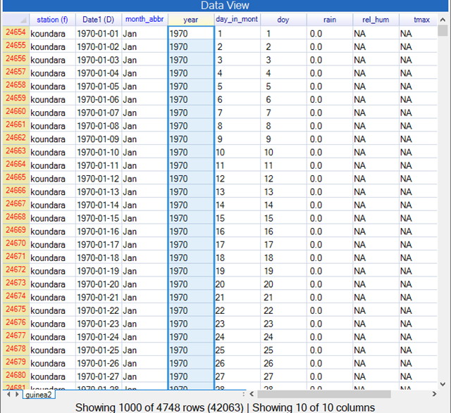
In Fig. 11 the first column is now in red, to indicate a filter is in operation. The data now starts with Koundara. Fig. 11 also indicates that just 4748 rows of data (out of the 42063 rows) have been selected for this stage in the analysis.

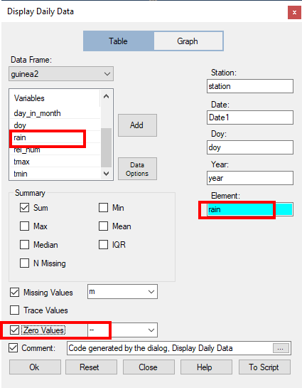
• Choose Climatic > Check Data, as in Fig. 1 and choose the second option, Display Daily.
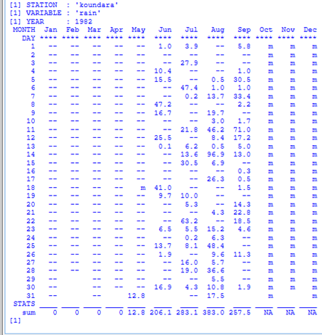
• Choose to display the rainfall data, and complete the dialogue as shown in Fig. 12.

One year of the data is shown in Fig. 13, with the zero values and missing data shown clearly.

Fig. 12 The display daily data dialogue	Fig. 13 One year of the data

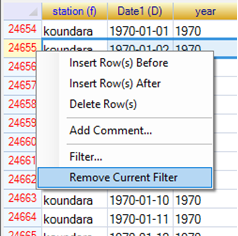
We remove the filter before our next check on the data.

• Either go into the name field, Fig. 6 and choose the last option Remove Current Filter. Or go to the left-hand column (the one in red), Fig. 14, right-click and choose Remove Current Filter.

Fig. 14 Right-click in the rows	Fig. 15 Choosing boxplots

Boxplots are a useful way to explore the data and to check for data quality at the same time.

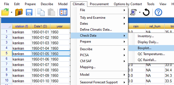
• Use Climatic > Check Data > Boxplots as shown in Fig. 15.
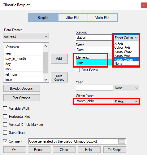
• Complete the dialogue as shown in Fig. 16, so change the data to tmax, give 2 columns (facets) for the stations and show the seasonal pattern through plotting by Months.

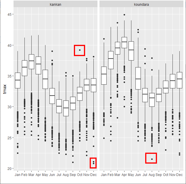
The result is shown in Fig. 17. The seasonal pattern is clear with the hottest months being March and April, and with Koundara being hotter then compared to Kankan. There are also some surprising values to be investigated further and this is done later. A few are marked in red in Fig. 17.

Fig. 16 Boxplots by month for tmax	Fig. 17 The seasonal pattern

An alternative is to plot the data by year, i.e. in time-series order.

• Return to the last (climatic boxplot) dialogue.
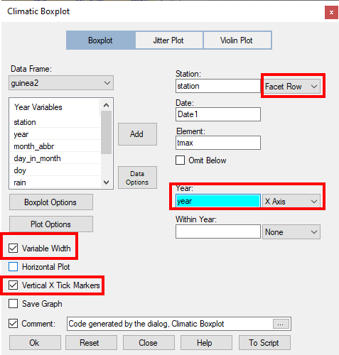
• In Fig. 18 change the x-axis to the year column. Make the boxplots of variable width and also make the x-axis labels vertical. Change the Station from Facet Column, to Facet Row.

Fig. 18 Boxplots by year for tmax	Fig. 19 Boxplots by month for rain

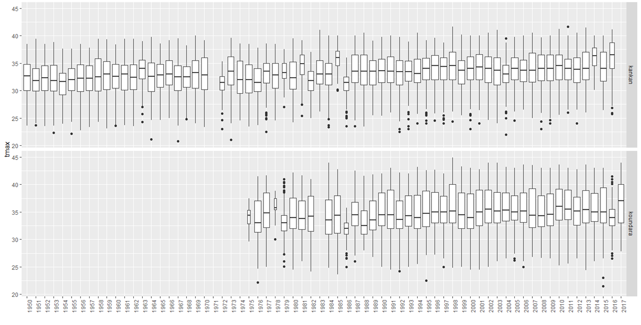The result is shown below, Fig. 20.
Many other options are possible, but we illustrate with just one more

• Return to the last dialogue.
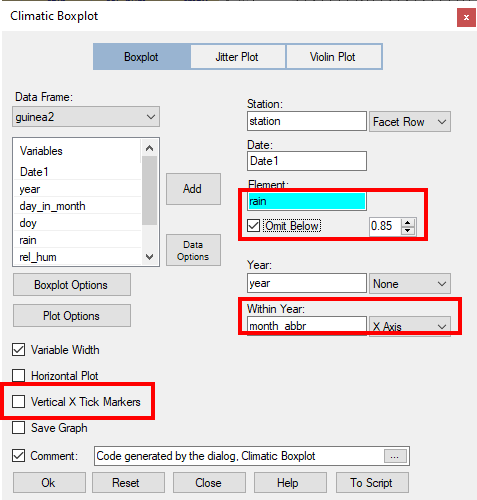
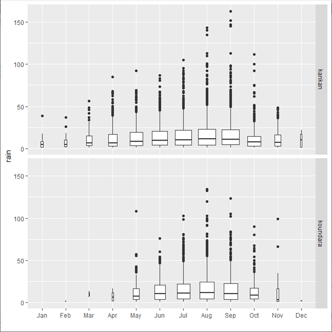
• In Fig. 19, change the variable to the rain column and tick the box to omit zero rainfalls. Make the month into the x-axis again. The x-tick markers do not need to be vertical.
• Press Ok to give the results shown in Fig. 21. They show that the overall pattern of seasonality is the same. Kankan do have occasional rain in the December to March period, but this is very rare in Koundara.

Fig. 20 Boxplots for tmax	Fig. 21 Boxplots on rain days

Finally, in the Check data menu, we use the quality control dialogues. This is illustrated with checks for the temperature data.

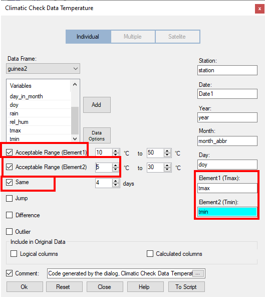
• Use Climatic > Check Data > QC Temperatures. This dialogue is designed particularly for checks for tmax and tmin, though it can be used for any temperature data.
• Put tmax and tmin into the respective field, see Fig. 22.
• Tick the first 2 boxes and change the lower limit for tmin (Element 2) to 5 degrees.
• The third option checks if 4 or more successive values of either tmax or tmin are the same value. Check this option also, see Fig. 22, leaving the option at the default value of 4 days

Fig. 22 Initial checks	Fig. 23 Two further sets of checks

When you press Ok the results are put into another data frame, which is called qcTemp, see Fig. 24, below.
Before explaining the results, we conduct further checks.

• Return to the last dialogue.
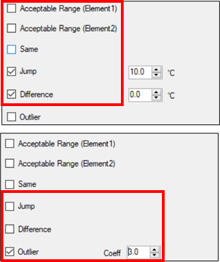
• Uncheck the three options from Fig. 22 and check the next 2, called Jump and Difference.

The jump option shows days when the day-to-day difference for tmax, or tmin is large. The default is 10 degrees. The difference option compares tmax with tmin and the default is to show all days when the difference is less than or equal to zero.

• Press Ok and you see that the results go into a further data frame, called qcTemp1.
• Return to the same dialogue again.
• Untick Jump and Difference and check the box for Outlier.
• Change the Outlier value from 1.5 (the default for a boxplot) to 3.
• Press Ok to produce the filtered values in a new data frame called qcTemp2. Now examine the resulting data frames in turn.

Fig. 24 Results from the range and repeated values checks

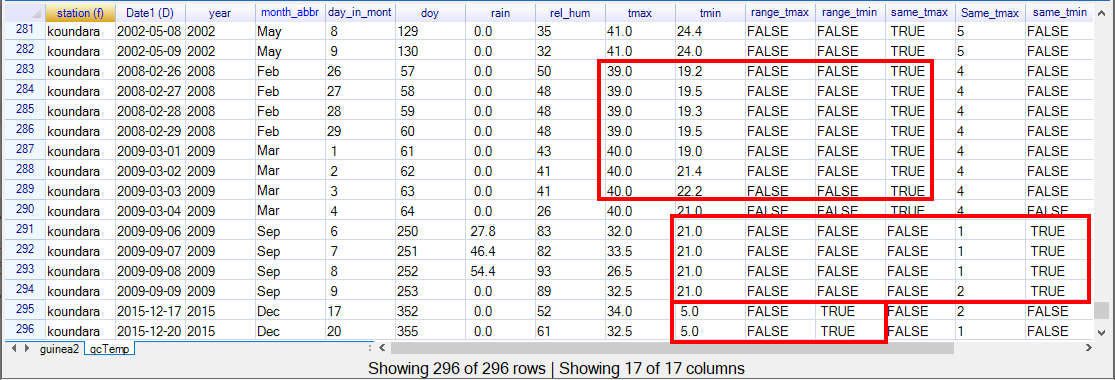
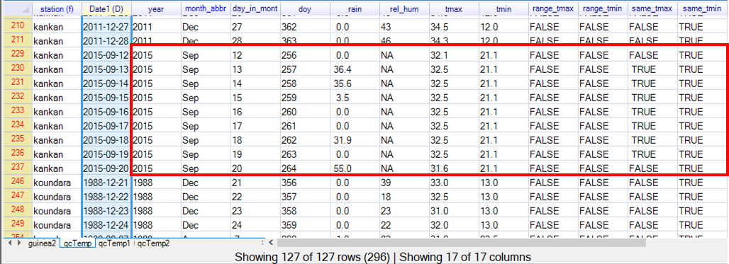
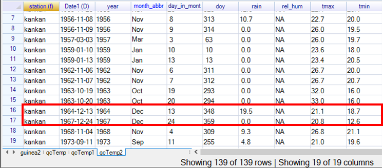
Part of the first data frame, called qcTemp, is given above, Fig. 24.
There are 296 values to examine. The last 2 rows, in the red box, at the bottom of Fig. 24 are December 17th and 20th 2015 and are the only occasions when the temperatures were out of the range, and they were minimum temperatures of just 5 degrees. The 4 rows above are September 6 to 9 2009 with a minimum temperature always 21.0 degrees.
The 8 rows above are February 26 to 29 2008, with a tmax of 39.0 degrees, and then Match 1 to 4 has tmax of 40.0 degrees.
One further feature of the “system” in R-Instat is that a logical column has been produced for each test, as shown in Fig. 24. This is TRUE for each day where the condition was not satisfied. This makes it easy to filter to investigate an individual condition in more detail. As an example we filter the data frame to look at the successive days when tmin was the same.
We filtered before – see Fig. 6 and the following figures, so the ideas below should be familiar.

• Make sure you are in the data frame called qcTemp.
• Then right click in the name row at the top and choose the option Filter.
• In the subsequent dialogue choose the button Define new filter.
• In the resulting sub-dialogue choose the column called same_tmin.
• Make the condition that same_tmin == TRUE.
• Rename the filter to be sameTmin.
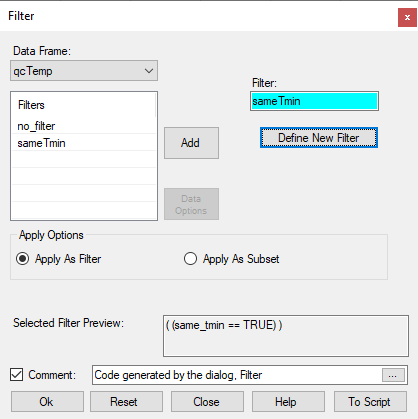
• Press Return to return to the main Filter dialogue, see Fig. 25.
• Press Ok and you see the first column in the data frame has turned red, to indicate a filter is in operation.

Fig. 25 A filter for tmin	Fig. 26 When tmin is identical on successive days

From Fig. 26 we see there are now just 139 days to investigate. In Fig. 26 we have marked one interesting feature. In Kankan in September 2015 there are as many as 9 successive days when tmin was recorded as 21.1 degrees. Also, on 7 of those days, the logical column for tmax was also TRUE, i.e. tmax was recorded as 32.5 degrees on each day. We now look briefly at the results from the other checks, shown in Fig. 27 and Fig. 28.

Fig. 27 Jumps between days or tmax <= tmin	Fig. 28 Outliers in tmax or tmin

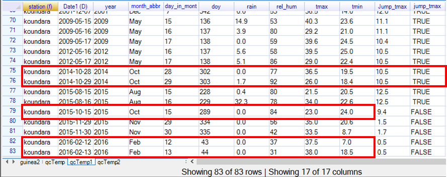
In Fig. 27 tmax was 36.5 degrees C on October 28 2014 and 26.0 on the following day, a difference of 10.5 degrees. The second example indicated in Fig 27 was the only occasion in the record when tmax was less than tmin, which was on October 15th 2015. The third example indicated was a jump from 7 degrees to 18.5 degrees on February 12 and 13th 2016.
Fig 28 shows outliers using similar criteria to those in the boxplots, shown earlier in Fig 17 and 18. In Fig. 28 we have marked 2 days in December 1964 and 1967, where tmax was low. These days were also marked as likely to need investigation in Fig. 17 earlier.
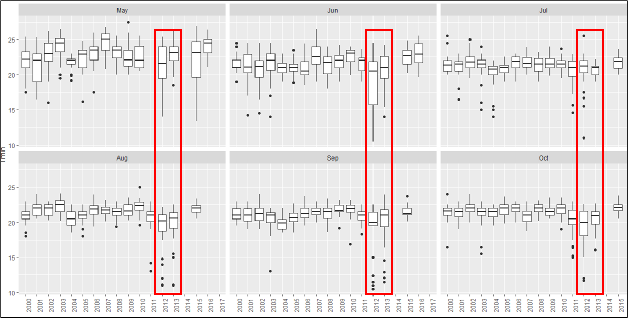
Finally, one surprise in the data frame of the outliers was that 39 of the 139 outliers were from tmin in Kankan in the Summer months of 2012 and 2013. This was not obvious from boxplots of the type shown earlier. We leave as a challenge the detailed steps needed (filter plus boxplot) to produce the boxplot by year and month together, shown in Fig. 29.

Fig. 29 Boxplots by year and month to examine outliers