Continuous Data

Continuous Data Example

Matt Wheeler Ph.D. 4/26/2023

Basics of Toxic R Continuous run.

This file shows ToxicR for dichotomous benchmark dose analyses using both single model and multiple model fits. The first thing we need to do is load the data. From an excel file this can be done using the following R commands:

cont_data           <- matrix(0,nrow=5,ncol=4)
colnames(cont_data) <- c("Dose","Mean","N","SD")
cont_data[,1] <- c(0,50,100,200,400)
cont_data[,2] <- c(5.26,5.76,6.13,8.24,9.23)
cont_data[,3] <- c(20,20,20,20,20)
cont_data[,4]<-  c(2.23,1.47,2.47,2.24,1.56)
Y <- cont_data[,2:4]

Hill fit

In what follows, I describe fitting the models using summary statistics. One can also fit these models using the original data with no change to the function call except the Y is a $n\times 1$ now one column vector, and the dose vector is also $n\times 1$ and corresponds to each entry in the data vector.

When summary data are used, ToxicR expects to be a $n\times 3$ matrix. The first column of is the the mean, the second colunn is the number of units on test, and the third column is the observed standard deviation. In what follows, lets look at the Hill model fit, where the Hill model is

library(ToxicR)
#> 
#> 
#>   _______               _____
#>  |__   __|      🤓     |  __ \
#>     | | _____  ___  ___| |__) |
#>     | |/ _ \ \/ / |/ __|  _  /
#>     | | (_) >  <| | (__| | \ \
#>     |_|\___/_/\_\_|\___|_|  \_\
#>                            23.4.1.1.0
#>     ___
#>     | |
#>     / \                   ____()()
#>    /☠☠☠\                 /       xx
#>   (_____)          `~~~~~\_;m__m.__>o
#> 
#> 
#> THE SOFTWARE IS PROVIDED AS IS, WITHOUT WARRANTY OF ANY KIND, EXPRESS OR IMPLIED,
#> INCLUDING BUT NOT LIMITED TO THE WARRANTIES OF MERCHANTABILITY, FITNESS FOR A
#> PARTICULAR PURPOSE AND NONINFRINGEMENT. IN NO EVENT SHALL THE AUTHORS OR COPYRIGHT
#> HOLDERS BE LIABLE FOR ANY CLAIM, DAMAGES OR OTHER LIABILITY, WHETHER IN AN ACTION OF
#> CONTRACT, TORT OR OTHERWISE, ARISING FROM, OUT OF OR IN CONNECTION WITH THE SOFTWARE
#> OR THE USE OR OTHER DEALINGS IN THE SOFTWARE.
library(ggplot2)
hill_fit <- single_continuous_fit(cont_data[,"Dose"],Y,
                                  model_type="hill")

Object Extraction

The last line fits the Hill Bayesian Laplace model and puts all of the information one needs in the `hill_fit’ object variable. This variable has the same structure as its dichotomous counterpart. By default the procedure assumes normal variance proportional to the mean. To see what model you fit, simply type the following line:

hill_fit$full_model
#> [1] "Model: Hill Distribution: Normal-NCV"
hill_fit$prior
#> Hill Model [normal-ncv]  Parameter Priors
#> ------------------------------------------------------------------------
#> Prior [a]:Normal(mu = 1.00, sd = 1.000) 1[-100.00,100.00]
#> Prior [b]:Normal(mu = 0.00, sd = 1.000) 1[-100.00,100.00]
#> Prior [c]:Log-Normal(log-mu = 0.00, log-sd = 2.000) 1[0.00,100.00]
#> Prior [d]:Log-Normal(log-mu = 0.47, log-sd = 0.421) 1[0.00,18.00]
#> Prior [rho]:Log-Normal(log-mu = 0.00, log-sd = 1.000) 1[0.00,100.00]
#> Prior [log(sigma^2)]:Normal(mu = 0.83, sd = 1.000) 1[-18.00,18.00]

Here, we see the Hill model is fit using the Normal-NCV, or normal variance proportional to the mean. For the Hill model, you can also use ‘normal’ as a distribution option.

hill_fit <- single_continuous_fit(cont_data[,"Dose"],
                                  cbind(cont_data[,"Mean"],cont_data[,"N"],cont_data[,"SD"]),
                                  model_type="hill",distribution = "normal",
                                  fit_type = "mcmc")
hill_fit$full_model
#> [1] "Model: Hill Distribution: Normal"
plot(hill_fit)

Notice how the `distribution’ option controls the distribution. For the “hill”, “power”, and “polynomial” DR models you can choose either “normal” or “normal-ncv.” or the “exp-3” and “exp-5” models you can also choose “lognormal.”

exp5_fit <- single_continuous_fit(cont_data[,"Dose"],Y,
                                  model_type="exp-5",distribution = "lognormal",fit_type="laplace")
exp5_fit$full_model
#> [1] "Model: Exponential-5 Distribution: Log-Normal"
plot(exp5_fit)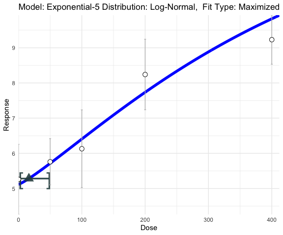

Benchmark Dose Types

Absolute Deviation

There are also other types of BMDs you can choose. Here one can specify absolute deviation as ‘abs,’ which solves where BMR is a specific cutoff value. In the example below, the abosolute difference of $\mbox{BMR} = 2.$

hill_sd_fit <- single_continuous_fit(cont_data[,"Dose"],Y,
                                  model_type="hill",distribution = "normal-ncv", fit_type="mcmc",
                                  BMD_TYPE="abs",BMR = 2)
#> Warning in single_continuous_fit(cont_data[, "Dose"], Y, model_type = "hill", :
#> BMD_TYPE is deprecated. Please use BMR_TYPE instead
hill_sd_fit$full_model
#> [1] "Model: Hill Distribution: Normal-NCV"
plot(hill_sd_fit)

Standard Deviation

The standard deviation approach is the default approach, and this is the value that solves and in this definition the $BMR \geq 0$ is the number of standard deviations the mean changes from no-exposure. In the example below, the $\mbox{BMR} = 1.5.$

hill_sd_fit <- single_continuous_fit(cont_data[,"Dose"],
                                  cbind(cont_data[,"Mean"],cont_data[,"N"],cont_data[,"SD"]),
                                  model_type="hill",distribution = "normal-ncv",fit_type="laplace",
                                  BMD_TYPE="sd",BMR = 1.5)
#> Warning in single_continuous_fit(cont_data[, "Dose"], cbind(cont_data[, :
#> BMD_TYPE is deprecated. Please use BMR_TYPE instead
hill_sd_fit$full_model
#> [1] "Model: Hill Distribution: Normal-NCV"
plot(hill_sd_fit)

Hybrid Deviation

The hybrid approach is a probabilistic approach that mimics risk for dichotomous data. Here, the BMD is the value that solves Here, $Pr[y > Y_0 \mid 0]$ is the probability that an ‘adverse’ response is observed at background dose, and $0 < \mbox{BMR} < 1$ is the increase in probability of seeing an adverse response at dose $\mbox{BMD}$ . For this approach $Pr[y < Y_0 \mid 0]$ must be specified using the “point_p” option. This option is only used when “hybrid” is specified. The following shows a Hill fit, where the BMD with only a $2.5\%$ chance of being observed at no dose, but has a $12.25\%$ probability of being observed at dose $\mbox{BMD}.$ Note: $\frac{0.1225 - 0.025}{0.975} = 0.1.$ For more information on this approach see Crump [@crump1995calculation].

hill_hybrid_fit <- single_continuous_fit(cont_data[,"Dose"],
                                  cbind(cont_data[,"Mean"],cont_data[,"N"],cont_data[,"SD"]),
                                  model_type="hill",distribution = "normal-ncv",fit_type="mcmc",
                                  BMD_TYPE="hybrid",point_p = 0.025,BMR = 0.1)
#> Warning in single_continuous_fit(cont_data[, "Dose"], cbind(cont_data[, :
#> BMD_TYPE is deprecated. Please use BMR_TYPE instead
hill_hybrid_fit$full_model
#> [1] "Model: Hill Distribution: Normal-NCV"
plot(hill_hybrid_fit)

Relative Deviation

The relatived deviation approach [@slob2002dose] is the value that solves

where $\mbox{BMR} > 0$ is the value of increase/decrease from the background.

hill_rd_fit <- single_continuous_fit(cont_data[,"Dose"],
                                  cbind(cont_data[,"Mean"],cont_data[,"N"],cont_data[,"SD"]),
                                  model_type="hill",distribution = "normal-ncv", fit_type="mcmc",
                                  BMD_TYPE="rel",BMR = 0.1,samples = 50000)
#> Warning in single_continuous_fit(cont_data[, "Dose"], cbind(cont_data[, :
#> BMD_TYPE is deprecated. Please use BMR_TYPE instead
hill_rd_fit$full_model
#> [1] "Model: Hill Distribution: Normal-NCV"
plot(hill_rd_fit)

Note: The above definitions are for for increasing data, `ToxicR’ will determine the direction of adversity and adjust computations accordingly.

Prior Specification

Like the dichotomous case you can modify the priors, to see what prior you want to modify Again, this is easy we can type the following code to see what our current prior is:

hill_sd_fit$prior
#> Hill Model [normal-ncv]  Parameter Priors
#> ------------------------------------------------------------------------
#> Prior [a]:Normal(mu = 1.00, sd = 1.000) 1[-100.00,100.00]
#> Prior [b]:Normal(mu = 0.00, sd = 1.000) 1[-100.00,100.00]
#> Prior [c]:Log-Normal(log-mu = 0.00, log-sd = 2.000) 1[0.00,100.00]
#> Prior [d]:Log-Normal(log-mu = 0.47, log-sd = 0.421) 1[0.00,18.00]
#> Prior [rho]:Log-Normal(log-mu = 0.00, log-sd = 1.000) 1[0.00,100.00]
#> Prior [log(sigma^2)]:Normal(mu = 0.83, sd = 1.000) 1[-18.00,18.00]

prior <- create_prior_list(normprior(0,1,-100,100),
                           normprior(0,1,-1e4,1e4),
                           lnormprior(0,1, 0, 100),
                           lnormprior(log(1),0.4215,0,18),
                           lnormprior(0,1,0,100),
                           normprior(0, 10,-100,100));

p_hill_ncv = create_continuous_prior(prior,"hill","normal-ncv")

prior <- create_prior_list(normprior(0,1,-100,100),
                           normprior(0,1,-1e4,1e4),
                           lnormprior(0,1, 0, 100),
                           lnormprior(log(1),0.4215,0,18),
                           normprior(0, 10,-100,100));

p_hill_norm = create_continuous_prior(prior,"hill","normal")

When specifying a prior, it is slightly different than the dichotomous case. Here, we need to specify what distribution we are using too. This adds one or two parameters depending on the parameters. All models have a parameter called $\log(\sigma^2),$ which is the variance term, and it is ALWAYS the last parameter in the model, and the
prior is placed over the log of this value. For the ‘normal-NCV’ option, the variance is $\sigma^2 f(dose)^\rho,$ i.e., it has an additional parameter $\rho.$ The parameter $\rho$ must have a prior, which is $\mbox{log-Normal}(0,1)$ in the above code.

hill_sd_a_fit <- single_continuous_fit(cont_data[,"Dose"],
                                  cbind(cont_data[,"Mean"],cont_data[,"N"],cont_data[,"SD"]),
                                  prior=p_hill_ncv,
                                  fit_type="laplace",
                                  BMD_TYPE="sd",BMR = 1.5)
#> Warning in single_continuous_fit(cont_data[, "Dose"], cbind(cont_data[, :
#> BMD_TYPE is deprecated. Please use BMR_TYPE instead

hill_sd_b_fit <- single_continuous_fit(cont_data[,"Dose"],
                                  cbind(cont_data[,"Mean"],cont_data[,"N"],cont_data[,"SD"]),
                                  prior=p_hill_norm,
                                  fit_type="laplace",
                                  BMD_TYPE="sd",BMR = 1.5)
#> Warning in single_continuous_fit(cont_data[, "Dose"], cbind(cont_data[, :
#> BMD_TYPE is deprecated. Please use BMR_TYPE instead

library(ggpubr)
figure <- ggarrange(plot(hill_sd_a_fit)+ggtitle(""), 
                    plot(hill_sd_b_fit)+ggtitle(""),
                    labels = c("Prior NCV", "Prior Normal"),
                    ncol = 1, nrow = 2)

figure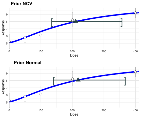

In the above code, we didn’t need to specify the ‘model_type’ or ‘distribution’ because this is done implicitly when you specify the prior. The above code works for the hill model, lets try it for a polynomial model.

poly_sd <- single_continuous_fit(cont_data[,"Dose"],Y,
                                  distribution="normal",model_type="polynomial",
                                  degree = 4, 
                                  fit_type="laplace",
                                  BMD_TYPE="sd",BMR = 0.5)
#> WARNING: Polynomial models may provide unstable estimates because of possible non-monotone behavior.
#> Warning in single_continuous_fit(cont_data[, "Dose"], Y, distribution =
#> "normal", : BMD_TYPE is deprecated. Please use BMR_TYPE instead

plot(poly_sd)

Model Averaging

Beyond single model fits, one can also use model averging for continuous models. As a default 10 models are fit. Here, the ‘hill’ and ‘power’ options are fit under the ‘normal’ and ‘normal-ncv’ distribution assumptions. Additionally to the ‘normal’ and ‘normal-ncv’ distributions the ‘exp-3’ and ‘exp-5’ also use the ‘lognormal’ distribution. Note that the polynomial model is not used because of constraint issues.

ma_sd_mcmc <- ma_continuous_fit(cont_data[,"Dose"],Y, fit_type="mcmc",
                             BMD_TYPE="sd",BMR = 0.5,samples = 50000)
#> Warning in ma_continuous_fit(cont_data[, "Dose"], Y, fit_type = "mcmc", :
#> BMD_TYPE is deprecated. Please use BMR_TYPE instead

ma_sd_laplace <- ma_continuous_fit(cont_data[,"Dose"],Y, fit_type="laplace",
                                   BMD_TYPE="sd",BMR = 0.5)
#> Warning in ma_continuous_fit(cont_data[, "Dose"], Y, fit_type = "laplace", :
#> BMD_TYPE is deprecated. Please use BMR_TYPE instead

plot(ma_sd_mcmc)
#> Scale for x is already present.
#> Adding another scale for x, which will replace the existing scale.

summary(ma_sd_laplace)
#> Summary of single MA BMD
#> 
#> Individual Model BMDS
#> Model                                                                     BMD (BMDL, BMDU)   Pr(M|Data)
#> ___________________________________________________________________________________________
#> Logistic-Aerts Distribution: Normal                                      83.83 (45.11 ,135.72)    0.178
#> Probit-Aerts Distribution: Normal                                        86.91 (47.50 ,134.81)    0.144
#> LMS Distribution: Log-Normal                                             80.72 (42.66 ,172.08)    0.112
#> Logistic-Aerts Distribution: Log-Normal                                  70.06 (32.38 ,130.14)    0.101
#> Exponential-Aerts Distribution: Log-Normal                               70.86 (32.02 ,136.19)    0.068
#> Probit-Aerts Distribution: Log-Normal                                    75.77 (36.90 ,125.07)    0.068
#> Gamma-EFSA Distribution: Log-Normal                                      55.65 (21.31 ,111.81)    0.052
#> Gamma-EFSA Distribution: Normal                                          67.07 (29.97 ,122.22)    0.046
#> Exponential-Aerts Distribution: Normal                                   82.46 (42.23 ,142.67)    0.044
#> Hill-Aerts Distribution: Log-Normal                                      70.01 (34.68 ,118.87)    0.040
#> Inverse Exponential-Aerts Distribution: Normal                           106.96 (67.79 ,145.12)   0.032
#> Lognormal-Aerts Distribution: Normal                                     98.03 (56.37 ,152.66)    0.031
#> Lognormal-Aerts Distribution: Log-Normal                                 87.75 (46.03 ,147.16)    0.029
#> Inverse Exponential-Aerts Distribution: Log-Normal                       106.12 (55.00 ,145.95)   0.027
#> Hill-Aerts Distribution: Normal                                          80.76 (43.98 ,127.61)    0.027
#> LMS Distribution: Normal                                                 133.08 (124.95 ,142.68)      0.001
#> ___________________________________________________________________________________________
#> Model Average BMD: 80.46 (37.81, 143.23) 90.0% CI
cleveland_plot(ma_sd_laplace)

MAdensity_plot(ma_sd_mcmc)
#> Picking joint bandwidth of 2.94

Here, ‘cleveland_plot’ and ‘MAdensity_plot’ can be used in the same way as in dichotomous plot. Like the dichotomous case, we can create a prior list for our model average.

prior <- create_prior_list(normprior(0,1,-100,100),
                           normprior(0,1,-1e4,1e4),
                           lnormprior(0,1, 0, 100),
                           lnormprior(log(1),0.4215,0,18),
                           lnormprior(0,1,0,100),
                           normprior(0, 10,-100,100));

p_hill_ncv = create_continuous_prior(prior,"hill","normal-ncv")

prior <- create_prior_list(normprior(0,1,-100,100),
                           normprior(0,1,-1e4,1e4),
                           lnormprior(0,1, 0, 100),
                           lnormprior(log(1),0.4215,0,18),
                           normprior(0, 10,-100,100));

p_hill_norm = create_continuous_prior(prior,"hill","normal")

prior <- create_prior_list(normprior(0,1,-100,100),
                           normprior(0,1,-1e4,1e4),
                           lnormprior(0,1, 0, 100),
                           lnormprior(log(1),0.4215,0,18),
                           normprior(0, 10,-100,100));

p_exp5_norm = create_continuous_prior(prior,"exp-5","normal")

prior <- create_prior_list(normprior(0,1,-100,100),
                           normprior(0,1,-1e4,1e4),
                           lnormprior(log(1),0.4215,0,18),
                           normprior(0, 10,-100,100));
p_power_norm = create_continuous_prior(prior,"power","normal")

prior <- create_prior_list(normprior(0,1,-100,100),
                           normprior(0,1,-1e4,1e4),
                           lnormprior(log(1),0.4215,0,18),
                           normprior(0, 10,-100,100));
p_exp3_norm = create_continuous_prior(prior,"exp-3","normal")
#> NOTE: Parameter 'c' added to prior list. It is not used in the analysis.
prior_list = list(p_exp3_norm,p_hill_norm,p_exp5_norm,p_power_norm)

With a list of priors one can then run a model average based upon a user specified model space. Here, all of the same benchmark dose options of ‘single_continuous_fit’ apply.

ma_sd_mcmc_2 <- ma_continuous_fit(cont_data[,"Dose"],Y, fit_type= "laplace",
                             BMD_TYPE="sd",BMR = 0.5,samples = 50000,model_list=prior_list)
#> Warning in ma_continuous_fit(cont_data[, "Dose"], Y, fit_type = "laplace", :
#> BMD_TYPE is deprecated. Please use BMR_TYPE instead
plot(ma_sd_mcmc_2)
#> Scale for x is already present.
#> Adding another scale for x, which will replace the existing scale.

References

Wout Slob, Dose-Response Modeling of Continuous Endpoints, Toxicological Sciences, Volume 66, Issue 2, April 2002, Pages 298–312

Crump, Kenny S., Calculation of benchmark doses from continuous data, Risk Analysis, Volume 15, Issue 1, February 1995, Pages 79-89

ToxicR

Installing

Installing

Provide feedback

Saved searches

Use saved searches to filter your results more quickly