Model training
The neural network model within the NanoVar SV calling pipeline functions to enrich true SV events based on read mapping characteristics and SV read support information. It provides a score for each SV which advises the confident level of its validity . This model was trained using simulated long-reads generated from a genome with simulated SVs. The model is applicable to real data assuming that the characteristics of real long-reads (e.g. error rate, indels) or genome (e.g . repetitive sequence proportions) are not vastly different from that of simulations. As the simulated long read characteristics were modeled after Oxford Nanopore Technologies (ONT) MinION long reads from a human genome, we believe that the model would be applicable to at least ONT reads sequenced from a human genome. In situations where the model would be less effective, such as using reads from a novel long-read sequencer, we have provided this tutorial for users to train their own model based on the characteristics of their own reads and genome of their organism of interest. We have also provided a brief model assessing method upon training completion and instructions on how to integrate the new model into NanoVar.
The usage of a custom-built model in NanoVar might improve or worsen SV calling precision. An improvement is not guaranteed. This venture is entirely exploratory based on your own data, and the authors of NanoVar are not liable to any possible performance decline or time forfeited as a result. Please proceed with this lengthy tutorial at your own discretion.
- NanoVar (>= v1.3.0)
- RSVSim (Only required for Stage A, see below)
- FASTX-Toolkit (fasta_formatter)
- bedtools
- pybedtools
- NanoSim OR your own long-read simulation software
- minimap2 (Required for NanoSim)
- numpy
- matplotlib
- tensorflow (>= 2.0.0)
- Scripts and data in the './scripts/model_toolkit' directory of NanoVar on GitHub
- Reference genome in FASTA (Please remove any scaffold or unknown contigs and use only main contigs (i.e. chr1 to chrY for hg38).
- 500k to 2 million real long-reads in FASTA/FASTQ to be used for error model building (only if you use NanoSim for read simulation)
- Pre-built SV genomes from here (only if you want to skip Stage A)
Stage A: SV genome simulation for training and test datasets (OPTIONAL)
This stage generates simulated SV genomes for the training and test datasets which can be skipped if you choose to use the pre-built SV genomes provided here which were configured with the default parameters described in this tutorial.
For each dataset, three genomes will be generated comprising of different subsets of the the same group of simulated SVs to assist the creation of mix zygosity SVs. Homozygous or heterozygous SVs will be produced when long-reads are simulated from these genomes at specific proportions. For example , we can simulate 10,000 SVs in Genome A, a subset of 8,000 SVs in Genome B, and a subset of 4,000 SVs in Genome C . The 4,000 SVs in Genome C are a subset of the 8,000 SVs in Genome B. Next, we can simulated 2.5 million reads from Genome A, 2.5 million reads from Genome B and 5 million reads from Genome C. By combining all reads into a 10 million reads FASTA and mapping it to the reference genome, we will have created 4,000 homozygous SV (B∩C), 4,000 heterozygous SV (B∩C'), and 2,000 low-coverage SVs (A∩B'). A homozygous SV only has SV -supporting reads at their breakends while a heterozygous SV has both SV-supporting and SV-opposing reads at similar proportions. A low-coverage SV will have mostly SV-opposing reads with usually only one or two SV-supporting reads.
Stage B: Long-read simulation using SV genomes
This stage simulates long-reads from the SV genomes created in Stage A. For long read simulation, you should use any long-read simulation software which can produce long-read characteristics resembling that of your own real long reads. For ONT reads, NanoSim can be used for analysis and read simulation as utilized in this tutorial. The reads will be simulated from each SV genome at different proportions and combined to produce the effect of mixed-zygosity SVs after they are mapped to a reference genome. These reads will be used as input into NanoVar and run with the "--debug" option to produce several intermediate output files. These files will be used for the neural network model training and testing in stage C.
Stage C: Neural network model building and supervised learning
After running NanoVar on the simulated long-reads, we use the intermediate files as input data for training our neural network model. We first pre-process the intermediate files (i.e. parse1.tsv, parse2.tsv and cluster.tsv) for both training and test datasets using the "NN_model_prep.py" script provided in the "scripts" directory on NanoVar's GitHub repository. Next, we use the Python 3 command-line interpreter to build the model architecture and train the model with the processed data. This step requires several rounds of network parameter tweaking and accuracy evaluation to achieve the optimal model. Finally, the newly trained model can be integrated into NanoVar by specifying it using the "--model" option prior to running.
Stage A: Download or generate training and test genomes with simulated SVs
Download pre-built SV genomes from here and proceed to point 5 at Stage B.
OR
Build and customise your own SV genomes:
1. Simulate SV locations using a mock RSVSim run
2. Split CSV files to different SV proportions
3. Simulate SV genomes at different SV proportions using new CSV files
4. Repeat steps 1-3 with a different seed to create the test genome
Stage B: Simulate long-reads from SV genomes and generate NanoVar intermediate files
5. Simulate long-reads from the SV genomes to create the training and test datasets
6. Run NanoVar on the training and test datasets in --debug mode to generate intermediate files
Stage C: Build your neural network model and train it
7. Neural network model training and assessment using Tensorflow and Keras
8. Integrate model into NanoVar for real data implementation
Create training dataset directory and enter it
mkdir training_set
cd training_set
RSVSim can be installed using bioconductor here Proceed to generate simulated SVs using RSVSim
# Load RSVSim library
library(RSVSim)

# Define pseudorandom seed (Modify this to differentiate training and test datasets)
s = 100

# Define your simulation settings
delno = 20000  # Number of deletion SVs
insno = 20000  # Combined number of viral insertion and transposition SVs
dupno = 5000  # Number of tandem duplication SVs
invno = 10000  # Number of inversion SVs

# Estimate SV sizes from real data
delSizes = estimateSVSizes(n=delno, minSize=50, maxSize=10000, default="deletions", hist=FALSE)
insSizes = estimateSVSizes(n=insno, minSize=50, maxSize=10000, default="insertions", hist=FALSE)
tandSizes = estimateSVSizes(n=dupno, minSize=50, maxSize=10000, default="tandemDuplications", hist=FALSE)
invSizes = estimateSVSizes(n=invno, minSize=50, maxSize=10000, default="inversions", hist=FALSE)

# Load own genome of reference
refgenome = readDNAStringSet("/path/to/own/genome.fa", format="fasta")

# Define output directory
out_dir = "./"

# Run simulation
sim = simulateSV(output=out_dir, genome=refgenome, del=delno, ins=insno, invs=invno, dups=dupno, sizeDels=delSizes, sizeIns =insSizes, sizeInvs=invSizes, sizeDups=tandSizes, maxDups=1, percCopiedIns=0, bpFlankSize=20, percSNPs=0.25, indelProb=0.5, maxIndelSize=5, bpSeqSize=200, seed=s, verbose=TRUE)

# Exit R and proceed to step 2
q()
This step prepares the SV location files required for the actual SV genome simulation (Assuming default settings as in step 1).
# Separate the 20,000 insertions.csv into 10,000 for transposition (TPO) and viral insertion (INS) regions each
tail -n +2 insertions.csv | head -n 10000 | cut -f 2-8 | awk -F'\t' '{print $1"\t"$2"\t"$3"\t"$7"\t"$4"\t"$5}' > tpo_A.csv
tail -n +10002 insertions.csv | cut -f 1-8 > viral_ins.csv

# Use Python scripts "custom_ins_list_RSVSim.py" and "total_viral_genome.fa" FASTA to generate viral regions for insertion into regions specified in viral_ins.csv
python3 custom_ins_list_RSVSim.py total_viral_genome.fa viral_ins.csv 100 10000 1 ./

# Make subset TPO/INS regions for SV subset genomes B and C
head -n 8000 tpo_A.csv > tpo_B.csv
head -n 4000 tpo_A.csv > tpo_C.csv
cut -f 1-6 viral_ins_regions1.csv > viral_ins_regions1_A.csv
head -n 8000 viral_ins_regions1_A.csv > viral_ins_regions1_B.csv
head -n 4000 viral_ins_regions1_A.csv > viral_ins_regions1_C.csv

# Combine TPO and INS CSV files
cat viral_ins_regions1_A.csv tpo_A.csv > total_ins_A.csv
cat viral_ins_regions1_B.csv tpo_B.csv > total_ins_B.csv
cat viral_ins_regions1_C.csv tpo_C.csv > total_ins_C.csv

# Remove header and make subset regions for deletion, inversion and duplication CSV files
tail -n +2 deletions.csv | cut -f 2-5 > del_A.csv
tail -n +2 deletions.csv | head -n 16000 | cut -f 2-5 > del_B.csv
tail -n +2 deletions.csv | head -n 8000 | cut -f 2-5 > del_C.csv
tail -n +2 tandemDuplications.csv | cut -f 2-5 > dup_A.csv
tail -n +2 tandemDuplications.csv | head -n 4000 | cut -f 2-5 > dup_B.csv
tail -n +2 tandemDuplications.csv | head -n 2000 | cut -f 2-5 > dup_C.csv
tail -n +2 inversions.csv | cut -f 2-5 > inv_A.csv
tail -n +2 inversions.csv | head -n 8000 | cut -f 2-5 > inv_B.csv
tail -n +2 inversions.csv | head -n 4000 | cut -f 2-5 > inv_C.csv

# Concatenate viral FASTA (produced by "custom_ins_list_RSVSim.py" script) into genome
cat viral_ins_fasta1.fa /path/to/own/genome.fa > genome_viral.fa

# Make ground-truth BED file with 400 bp error distance from the precise breakend
tail -n +2 deletions.csv | awk '{print $2"\t"$3-400"\t"$3+400"\t"$5"\t"$1"^1\n"$2"\t"$4-400"\t"$4+400"\t"$5"\t"$1"^2"}' | bedtools sort -i - > deletions.bed
tail -n +2 inversions.csv | awk '{print $2"\t"$3-400"\t"$3+400"\t"$5"\t"$1"^1\n"$2"\t"$4-400"\t"$4+400"\t"$5"\t"$1"^2"}' | bedtools sort -i - > inversions.bed
tail -n +2 tandemDuplications.csv | awk '{print $2"\t"$3-400"\t"$3+400"\t"$5"\t"$1"^1\n"$2"\t"$4-400"\t"$4+400"\t"$5"\t"$1"^2"}' | bedtools sort -i - > tandemDuplications.bed
tail -n +2 insertions.csv | head -n 10000 | awk '{print $2"\t"$3-400"\t"$3+400"\t"$8"\t""DEL_"$1"^1\n"$2"\t"$4-400"\t"$4+400"\t"$8"\t""DEL_"$1"^2\n"$5"\t"$6-400"\t"$6+400"\t"$8"\t"$1}' | bedtools sort -i - > tpo.bed
awk '{print $5"\t"$6-400"\t"$6+400"\t"$8"\tv"$1}' viral_ins.csv | bedtools sort -i - > viralins.bed
cat deletions.bed inversions.bed tandemDuplications.bed tpo.bed viralins.bed | awk '{if ($2 < 0) print $1"\t0\t"$3"\t"$4"\t"$5; else print $0}' | bedtools sort -i - > gtruth_400.bed
Create directories for the different genomes
mkdir genomeA
mkdir genomeB
mkdir genomeC
Change directory to genomeA
cd genomeA
Simulate genomeA with RSVSim in R
# Load RSVSim library
library(RSVSim)

# Read the prepared CSV files
insrange = read.table("../total_ins_A.csv")
delrange = read.table("../del_A.csv")
duprange = read.table("../dup_A.csv")
invrange = read.table("../inv_A.csv")

# Process regions
knownInsertion = GRanges(IRanges(insrange$V2,insrange$V3), seqnames=insrange$V1, chrB=insrange$V5, startB=insrange$V6)
knownDeletion = GRanges(IRanges(delrange$V2,delrange$V3), seqnames=delrange$V1)
knownInversion = GRanges(IRanges(invrange$V2,invrange$V3), seqnames=invrange$V1)
knownDuplication = GRanges(IRanges(duprange$V2,duprange$V3), seqnames=duprange$V1)

# Set random vector
randomvector = c(FALSE, FALSE, FALSE, FALSE, TRUE)

# Load the viral genome reference
refgenome = readDNAStringSet("../genome_viral.fa", format="fasta")

# Run simulation
sim = simulateSV(output="./", genome=refgenome, regionsDel=knownDeletion, regionsIns=knownInsertion, regionsInvs =knownInversion, regionsDups=knownDuplication, maxDups=1, bpFlankSize=20, percSNPs=0.25, indelProb=0.5 , maxIndelSize=5, bpSeqSize=200, random=randomvector, verbose=TRUE)

# Exit R
q()
Remove viral FASTA from genome (requires fasta_formatter from FASTX-Toolkit )
fasta_formatter -i genome_rearranged.fasta -w 0 | perl -pe 's/(\.\d)\n/$1/g' | grep -v '>NC' > genomeA.fa
Change directory to genomeB
cd ../genomeB
Simulate genomeB with RSVSim in R
# Load RSVSim library
library(RSVSim)

# Read the prepared CSV files
insrange = read.table("../total_ins_B.csv")
delrange = read.table("../del_B.csv")
duprange = read.table("../dup_B.csv")
invrange = read.table("../inv_B.csv")

# Process regions
knownInsertion = GRanges(IRanges(insrange$V2,insrange$V3), seqnames=insrange$V1, chrB=insrange$V5, startB=insrange$V6)
knownDeletion = GRanges(IRanges(delrange$V2,delrange$V3), seqnames=delrange$V1)
knownInversion = GRanges(IRanges(invrange$V2,invrange$V3), seqnames=invrange$V1)
knownDuplication = GRanges(IRanges(duprange$V2,duprange$V3), seqnames=duprange$V1)

# Set random vector
randomvector = c(FALSE, FALSE, FALSE, FALSE, TRUE)

# Load the viral genome reference
refgenome = readDNAStringSet("../genome_viral.fa", format="fasta")

# Run simulation
sim = simulateSV(output="./", genome=refgenome, regionsDel=knownDeletion, regionsIns=knownInsertion, regionsInvs =knownInversion, regionsDups=knownDuplication, maxDups=1, bpFlankSize=20, percSNPs=0.25, indelProb=0.5 , maxIndelSize=5, bpSeqSize=200, random=randomvector, verbose=TRUE)

# Exit R
q()
Remove viral FASTA from genome
fasta_formatter -i genome_rearranged.fasta -w 0 | perl -pe 's/(\.\d)\n/$1/g' | grep -v '>NC' > genomeB.fa
Change directory to genomeC
cd ../genomeC
Simulate genomeC with RSVSim in R
# Load RSVSim library
library(RSVSim)

# Read the prepared CSV files
insrange = read.table("../total_ins_C.csv")
delrange = read.table("../del_C.csv")
duprange = read.table("../dup_C.csv")
invrange = read.table("../inv_C.csv")

# Process regions
knownInsertion = GRanges(IRanges(insrange$V2,insrange$V3), seqnames=insrange$V1, chrB=insrange$V5, startB=insrange$V6)
knownDeletion = GRanges(IRanges(delrange$V2,delrange$V3), seqnames=delrange$V1)
knownInversion = GRanges(IRanges(invrange$V2,invrange$V3), seqnames=invrange$V1)
knownDuplication = GRanges(IRanges(duprange$V2,duprange$V3), seqnames=duprange$V1)

# Set random vector
randomvector = c(FALSE, FALSE, FALSE, FALSE, TRUE)

# Load the viral genome reference
refgenome = readDNAStringSet("../genome_viral.fa", format="fasta")

# Run simulation
sim = simulateSV(output="./", genome=refgenome, regionsDel=knownDeletion, regionsIns=knownInsertion, regionsInvs =knownInversion, regionsDups=knownDuplication, maxDups=1, bpFlankSize=20, percSNPs=0.25, indelProb=0.5 , maxIndelSize=5, bpSeqSize=200, random=randomvector, verbose=TRUE)

# Exit R
q()
Remove viral FASTA from genome
fasta_formatter -i genome_rearranged.fasta -w 0 | perl -pe 's/(\.\d)\n/$1/g' | grep -v '>NC' > genomeC.fa
Create test dataset directory and enter it
mkdir test_set
cd test_set
Repeat step 1-3 to create the test genome. A different seed and different amounts of SVs can be simulated for the test dataset .
An example of step 1 and step 2 is shown below.
Step 1:
# Load RSVSim library
library(RSVSim)

# Define pseudorandom seed
s = 200

# Define your simulation settings
delno = 2000  # Number of deletion SVs
insno = 2000  # Combined number of viral insertion and transposition SVs
dupno = 500  # Number of tandem duplication SVs
invno = 1000  # Number of inversion SVs

# Estimate SV sizes from real data
delSizes = estimateSVSizes(n=delno, minSize=50, maxSize=10000, default="deletions", hist=FALSE)
insSizes = estimateSVSizes(n=insno, minSize=50, maxSize=10000, default="insertions", hist=FALSE)
tandSizes = estimateSVSizes(n=dupno, minSize=50, maxSize=10000, default="tandemDuplications", hist=FALSE)
invSizes = estimateSVSizes(n=invno, minSize=50, maxSize=10000, default="inversions", hist=FALSE)

# Load own genome of reference
refgenome = readDNAStringSet("/path/to/own/genome.fa", format="fasta")

# Define output directory
out_dir = "./"

# Run simulation
sim = simulateSV(output=out_dir, genome=refgenome, del=delno, ins=insno, invs=invno, dups=dupno, sizeDels=delSizes, sizeIns =insSizes, sizeInvs=invSizes, sizeDups=tandSizes, maxDups=1, percCopiedIns=0, bpFlankSize=20, percSNPs=0.25, indelProb=0.5, maxIndelSize=5, bpSeqSize=200, seed=s, verbose=TRUE)

# Exit R and proceed to step 2
q()
Step 2:
# Separate the 2,000 insertions.csv into 1,000 for transposition (TPO) and viral insertion (INS) regions each
tail -n +2 insertions.csv | head -n 1000 | cut -f 2-8 | awk -F'\t' '{print $1"\t"$2"\t"$3"\t"$7"\t"$4"\t"$5}' > tpo_A.csv
tail -n +1002 insertions.csv | cut -f 1-8 > viral_ins.csv

# Use Python scripts "custom_ins_list_RSVSim.py" and "total_viral_genome.fa" FASTA to generate viral regions for insertion into regions specified in viral_ins.csv
python3 custom_ins_list_RSVSim.py total_viral_genome.fa viral_ins.csv 200 1000 1 ./

# Make subset TPO/INS regions for SV subset genomes B and C
head -n 800 tpo_A.csv > tpo_B.csv
head -n 400 tpo_A.csv > tpo_C.csv
cut -f 1-6 viral_ins_regions1.csv > viral_ins_regions1_A.csv
head -n 800 viral_ins_regions1_A.csv > viral_ins_regions1_B.csv
head -n 400 viral_ins_regions1_A.csv > viral_ins_regions1_C.csv

# Combine TPO and INS CSV files
cat viral_ins_regions1_A.csv tpo_A.csv > total_ins_A.csv
cat viral_ins_regions1_B.csv tpo_B.csv > total_ins_B.csv
cat viral_ins_regions1_C.csv tpo_C.csv > total_ins_C.csv

# Remove header and make subset regions for deletion, inversion and duplication CSV files
tail -n +2 deletions.csv | cut -f 2-5 > del_A.csv
tail -n +2 deletions.csv | head -n 1600 | cut -f 2-5 > del_B.csv
tail -n +2 deletions.csv | head -n 800 | cut -f 2-5 > del_C.csv
tail -n +2 tandemDuplications.csv | cut -f 2-5 > dup_A.csv
tail -n +2 tandemDuplications.csv | head -n 400 | cut -f 2-5 > dup_B.csv
tail -n +2 tandemDuplications.csv | head -n 200 | cut -f 2-5 > dup_C.csv
tail -n +2 inversions.csv | cut -f 2-5 > inv_A.csv
tail -n +2 inversions.csv | head -n 800 | cut -f 2-5 > inv_B.csv
tail -n +2 inversions.csv | head -n 400 | cut -f 2-5 > inv_C.csv

# Concatenate viral FASTA (produced by "custom_ins_list_RSVSim.py" script) into genome
cat viral_ins_fasta1.fa /path/to/own/genome.fa > genome_viral.fa

# Make ground-truth BED file with 400 bp error distance from the precise breakend
tail -n +2 deletions.csv | awk '{print $2"\t"$3-400"\t"$3+400"\t"$5"\t"$1"^1\n"$2"\t"$4-400"\t"$4+400"\t"$5"\t"$1"^2"}' | bedtools sort -i - > deletions.bed
tail -n +2 inversions.csv | awk '{print $2"\t"$3-400"\t"$3+400"\t"$5"\t"$1"^1\n"$2"\t"$4-400"\t"$4+400"\t"$5"\t"$1"^2"}' | bedtools sort -i - > inversions.bed
tail -n +2 tandemDuplications.csv | awk '{print $2"\t"$3-400"\t"$3+400"\t"$5"\t"$1"^1\n"$2"\t"$4-400"\t"$4+400"\t"$5"\t"$1"^2"}' | bedtools sort -i - > tandemDuplications.bed
tail -n +2 insertions.csv | head -n 1000 | awk '{print $2"\t"$3-400"\t"$3+400"\t"$8"\t""DEL_"$1"^1\n"$2"\t"$4-400"\t"$4+400"\t"$8"\t""DEL_"$1"^2\n"$5"\t"$6-400"\t"$6+400"\t"$8"\t"$1}' | bedtools sort -i - > tpo.bed
awk '{print $5"\t"$6-400"\t"$6+400"\t"$8"\tv"$1}' viral_ins.csv | bedtools sort -i - > viralins.bed
cat deletions.bed inversions.bed tandemDuplications.bed tpo.bed viralins.bed | awk '{if ($2 < 0) print $1"\t0\t"$3"\t"$4"\t"$5; else print $0}' | bedtools sort -i - > gtruth_400.bed
Step 3:
Refer to step 3 above.
In order to proceed with this stage, you need to have generated the SV genomes by either carrying out Stage A or download the pre-built SV genomes provided here.
For this step, please use your own long-read simulator suitable for the sequencing technology you work with. In this tutorial, NanoSim will be used to simulate long-reads from Oxford Nanopore Technologies (ONT) MinION.
Use NanoSim to analyse the characteristics of your real long-reads. You can create a subset of your FASTQ/FASTA file, about 500k-2 million reads should suffice. Note that the more reads you use, the longer the analysis will take.
# Run long-read analyzer
mkdir nanosim_model
cd nanosim_model
read_analysis.py genome -i real_ONT_data.fa -rg reference_genome.fa -t num_threads
Use NanoSim to generate simulated long-reads from SV genomes
# Change directory to genomeA (training_set)
cd genomeA

# Run simulator to generate 2.5 million reads from genomeA
simulator.py genome -rg genomeA.fa -c ../nanosim_model/training -o genomeA -n 2500000 --seed 100 -t num_threads
cat genomeA_aligned_reads.fasta genomeA_unaligned_reads.fasta > genomeA_reads.fasta

# Change directory to genomeB (training_set)
cd ../genomeB

# Run simulator to generate 2.5 million reads from genomeB
simulator.py genome -rg genomeB.fa -c ../nanosim_model/training -o genomeB -n 2500000 --seed 100 -t num_threads
cat genomeB_aligned_reads.fasta genomeB_unaligned_reads.fasta > genomeB_reads.fasta

# Change directory to genomeC (training_set)
cd ../genomeC

# Run simulator to generate 5 million reads from genomeC
simulator.py genome -rg genomeC.fa -c ../nanosim_model/training -o genomeC -n 5000000 --seed 100 -t num_threads
cat genomeC_aligned_reads.fasta genomeC_unaligned_reads.fasta > genomeC_reads.fasta

# Create combined directory and concatenate reads
cd ../
mkdir combined_ABC_train
cd combined_ABC_train
cat ../genomeA/genomeA_reads.fa ../genomeB/genomeB_reads.fa ../genomeC/genomeC_reads.fa > training_reads.fa


# Now same thing for the test data except with lesser reads (exact read number up to user)
# Change directory to genomeA (test_set)
cd genomeA

# Run simulator to generate 500k reads from genomeA
simulator.py genome -rg genomeA.fa -c ../nanosim_model/training -o genomeA -n 500000 --seed 200 -t num_threads
cat genomeA_aligned_reads.fasta genomeA_unaligned_reads.fasta > genomeA_reads.fasta

# Change directory to genomeB (test_set)
cd ../genomeB

# Run simulator to generate 500k reads from genomeB
simulator.py genome -rg genomeB.fa -c ../nanosim_model/training -o genomeB -n 500000 --seed 200 -t num_threads
cat genomeB_aligned_reads.fasta genomeB_unaligned_reads.fasta > genomeB_reads.fasta

# Change directory to genomeC (test_set)
cd ../genomeC

# Run simulator to generate 1 million reads from genomeC
simulator.py genome -rg genomeC.fa -c ../nanosim_model/training -o genomeC -n 1000000 --seed 200 -t num_threads
cat genomeC_aligned_reads.fasta genomeC_unaligned_reads.fasta > genomeC_reads.fasta

# Create combined directory and concatenate reads
cd ../
mkdir combined_ABC_test
cd combined_ABC_test
cat ../genomeA/genomeA_reads.fa ../genomeB/genomeB_reads.fa ../genomeC/genomeC_reads.fa > test_reads.fa
Please ensure you are using the latest version of NanoVar (>= 1.3.0).
# Change directory to combined_ABC_train (training_set)
cd combined_ABC_train

# Run NanoVar with --debug option on training reads
nanovar --debug -t num_threads -c 1 ./training_reads.fa /path/to/own/genome.fa ./nanovar

# Concatenate parsed files
cat nanovar/parse1.tsv nanovar/parse2.tsv > nanovar/parse_total.tsv


# Change directory to combined_ABC_test (test_set)
cd combined_ABC_test

# Run NanoVar with --debug option on test reads
nanovar --debug -t num_threads -c 1 ./test_reads.fa /path/to/own/genome.fa ./nanovar

# Concatenate parsed files
cat nanovar/parse1.tsv nanovar/parse2.tsv > nanovar/parse_total.tsv
Use the python script NN_model_prep.py to process NanoVar debug files from the training and test datasets
NN_model_prep.py script usage:
python3 NN_model_prep.py \
parse-train.tsv \
cluster-train.tsv \
gtruth_400-train.bed \
omit_region-train.bed \
parse-test.tsv \
cluster-test.tsv \
gtruth_400-test.bed \
omit_region-test.bed
| File | Remarks |
|---|---|
| parse-train.tsv | parse_total.tsv file from the training set |
| cluster-train.tsv | cluster.tsv file from the training set |
| gtruth_400-train.bed | gtruth_400.bed file from the training set |
| omit_region-train.bed | BED file of N-seq region junctions in the reference genome of training set. If using hg38, you can use the provided hg38_gap.bed or exclude_regions.bed. For other genomes, see below. |
| parse-test.tsv | parse_total.tsv file from the test set |
| cluster-test.tsv | cluster.tsv file from the test set |
| gtruth_400-test.bed | gtruth_400.bed file from the test set |
| omit_region-test.bed | BED file of N-seq region junctions in the reference genome of test set. If using hg38, you can use the provided hg38_gap.bed or exclude_regions.bed. For other genomes, see below. |
Usage example:
python3 NN_model_prep.py \
training_set/combined_ABC_train/nanovar/parse_total.tsv \
training_set/combined_ABC_train/nanovar/cluster.tsv \
training_set/gtruth_400.bed \
training_set/exclude_regions.bed \
test_set/combined_ABC_test/nanovar/parse_total.tsv \
test_set/combined_ABC_test/nanovar/cluster.tsv \
test_set/gtruth_400.bed \
test_set/exclude_regions.bed
Proceed to Stage C with the three files generated: test_set.txt, train0_set.txt, and train1_set.txt.
To generate a N-seq junction BED file for other genomes, download faToTwoBit and twoBitInfo from UCSC and follow these instructions:
# Convert reference genome to two bit
faToTwoBit genome.fa genome.2bit

# Generate N-seq junction BED file
twoBitInfo -nBed genome.2bit genome.2bit.nbed

# Create 400 bp buffer around N-seq junctions
awk -F'\t' '{print $1"\t"$2-400"\t"$3+400}' genome.2bit.nbed | awk -F'\t' '{if ($2<0) print $1"\t0\t"$3; else print $0 }' > genome_gap.bed
You can now use the genome_gap.bed file generated as the omit_region.bed file for the NN_model_prep.py script.
Build model in Python3 using Tensoflow and Keras modules
# Import modules
import random
import numpy as np
from tensorflow.keras.models import Sequential
from tensorflow.keras.layers import Dense, Activation
from tensorflow.keras.layers import Dropout
from tensorflow.keras.optimizers import SGD
import tensorflow as tf
import matplotlib.pyplot as plt


# Load files generated from NN_model_prep.py
train1 = []
train0 = []
test = []

with open('train1_set.txt') as f:
    for line in f:
        train1.append([float(x) for x in line.split(',')])

with open('train0_set.txt') as f:
    for line in f:
        train0.append([float(x) for x in line.split(',')])

with open('test_set.txt') as f:
    for line in f:
        test.append([float(x) for x in line.split(',')])


# Shuffle and split data array of test set
test_array = np.array(test, dtype=np.float64)
np.random.shuffle(test_array)
x_tests = np.split(test_array, [23], axis=1)[0]
y_tests = np.split(test_array, [23], axis=1)[1]


# Setting parameters (Modify to optimize model)
seed = 11
epoch = 380
batch = 100
sample_size = 8000


# Initialize random seeds
np.random.seed(seed)
random.seed(seed)
tf.random.set_seed(seed)


# Define model structure (Modify to optimize model)
model = Sequential()
model.add(Dense(12, input_dim=23, activation='relu'))
model.add(Dropout(0.4))
model.add(Dense(9, activation='relu'))
model.add(Dropout(0.3))
model.add(Dense(5, activation='relu'))
model.add(Dropout(0.2))
model.add(Dense(1, activation='sigmoid'))


# Compile model
model.compile(loss='binary_crossentropy', optimizer='SGD', metrics=['accuracy'])


# Define accuracy and loss list variables
acc = []
val_acc = []
loss = []
val_loss = []


# Fit the model
for i in range(epoch):
    # Sample equal number of truth and false entries and shuffle array
    train_set = random.sample(train1, sample_size) + random.sample(train0, sample_size)
    train_array = np.array(train_set, dtype=np.float64)
    np.random.shuffle(train_array)
    # Split array for input/output
    x_train = np.split(train_array, [23], axis=1)[0]
    y_train = np.split(train_array, [23], axis=1)[1]
    # Fit model
    fit = model.fit(x_train, y_train, epochs=1, batch_size=batch, validation_data=(x_tests, y_tests), verbose=1)
    # Record accuracy/loss for evaluation
    acc.append(fit.history['accuracy'])
    val_acc.append(fit.history['val_accuracy'])
    loss.append(fit.history['loss'])
    val_loss.append(fit.history['val_loss'])


# Plot model accuracy/loss for training and test set
fig = plt.figure()
ax = fig.add_subplot(111)
ax.plot(acc)
ax.plot(val_acc)
ax.plot(loss)
ax.plot(val_loss)
ax.set_ylim([0.0, 1.0])
plt.title('Model accuracy and loss')
plt.ylabel('Accuracy/Loss')
plt.xlabel('Epochs')
plt.legend(['train_accuracy', 'test_accuracy', 'train_loss', 'test_loss'], loc='upper left')
plt.show()

# Evaluate the model (See example plot below)

# If you are satisfied with the model's training, save the model
model.save('./my_model.h5', include_optimizer=False)
A somewhat good model training would look like this:
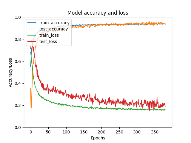
The overall gradual increase of train_accuracy and decrease of train_loss across epochs indicate that the training of the model had taken place. The plateau of both the accuracy and loss at high epochs implies that the training has reached its limits and that addition epochs might lead to over-training. The similar trends of test_accuracy and test_loss suggest good validation of the model on the test set. Users can modify the number of epochs, batch number, sample size and model structure to improve model training and performance. For more information about the neural network training, please visit Keras.
Once the model is created, it can be integrated into NanoVar using the --model option.
Example:
nanovar -t num_threads --model /path/to/my_model.h5 /path/to/reads.fa /path/to/genome.fa /path/to/working_dir
Congrats! You have made it to the end. In order to evaluate if your own model is better than the default model, we advice to run both models on our simulated SV benchmark datasets found here and compare their performances on a precision-recall plot.
I hope this tutorial was useful in improving your SV calling precision with NanoVar. Thank you for visiting and please raise an issue for any queries.