NanoVar report
The NanoVar report is a standalone HTML report that presents the run details, results summary, and quality control statistics of a NanoVar run. It is a convenient and quick way to visualize results and evaluate the credibility of a run. The report can be viewed using a web browser (e.g. Chrome, Firefox).
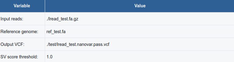
This table reports basic information such as the full paths to the input files (reads and reference genome), the path to the output "PASS" VCF file, and the SV score threshold used for the true SV enrichment.
 Click image to enlarge
This table contains characterized SV information for the top 1000 SVs in the "PASS" VCF file ranked by confidence score (Column 8). The table can be customized by display order according to any columns, or by searching for specific SVs using the search box. The customized table can be exported in CSV or MS Excel formats, or copied to clipboard as a tab-separated text. Below are descriptions of each column.
| Column # | Name | Description |
|---|---|---|
| 1 | # | A numerical index number for each SV. |
| 2 | SV type | Type of SV: Deletion (DEL), Insertion (INS), Tandem duplication (DUP), Inversion (INV), Other kinds of breakends (BND). |
| 3 | Chrom1 | Chromosome name of the left breakend of the SV. |
| 4 | Pos1 | Coordinate of the left breakend of the SV. |
| 5 | Chrom2 | Chromosome name of the right breakend of the SV. |
| 6 | Pos2 | Coordinate of the right breakend of the SV. |
| 7 | Length | Estimated length of SV in base pairs. |
| 8 | Score | Raw probability score before Phred conversion to QUAL confidence scores. |
| 9 | No. of breakend-sup reads | Number of long-reads supporting the/both breakend(s). |
| 10 | No. of breakend-opp reads | Number of long-reads NOT supporting the/both breakend(s). |
| 11 | Breakend read ratio | Calculated by Sup-reads/(Sup-reads + Opp-reads) |
| 12 | Approximated genotype | Approximate SV genotype (1/1 - Homozygous, 0/1 - Heterozygous). |
| 13 | SV ID | Assigned SV identification code which be used to search for its supporting reads in the sv_support_reads file (See Output). |
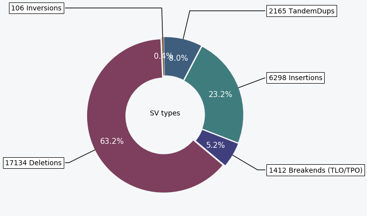
A donut chart showing the distribution of the different SV types characterized in the sample.
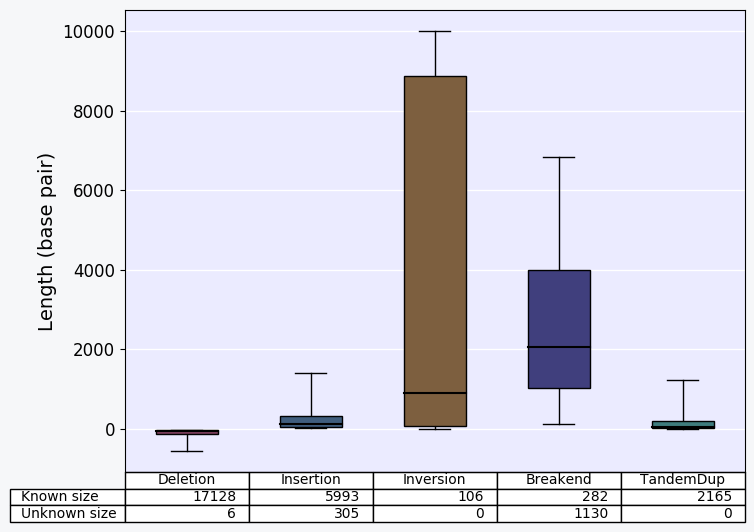
Bar-charts displaying the size distribution of each SV types for SVs characterized in the sample.
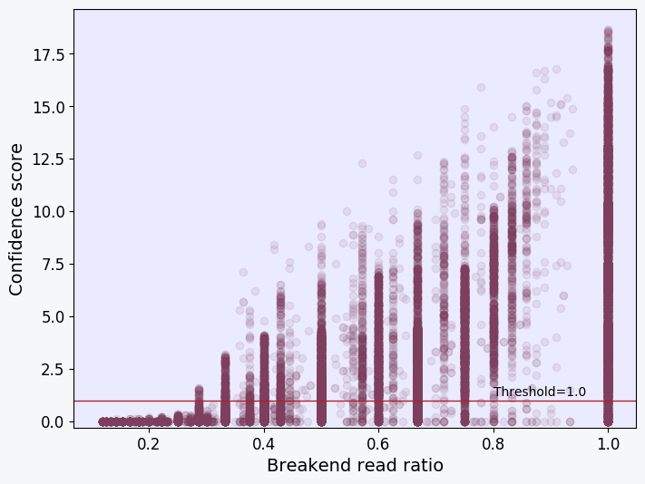
Scatter plot showing the confidence score and breakend read ratio of each SV characterized in the sample. Each point in the plot represents an SV. Generally, a positive correlation should be observed in the plot. SVs with a breakend read ratio of <0 .3 would usually have a confidence score of <2.6 and be removed from the "PASS" VCF file together with all other SVs that fall below the threshold score (red line).
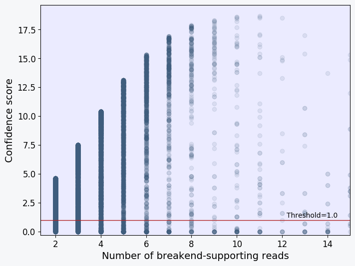
Scatter plot showing the confidence score and supporting read depth of each SV characterized in the sample. Each point in the plot represents an SV. The plot should show a positive correlation between the two variables. SVs with only a single breakend -supporting read should fall below the threshold value of 2.6 (red line) and be removed from the "PASS" VCF file together with all other SVs that fall below the threshold score.
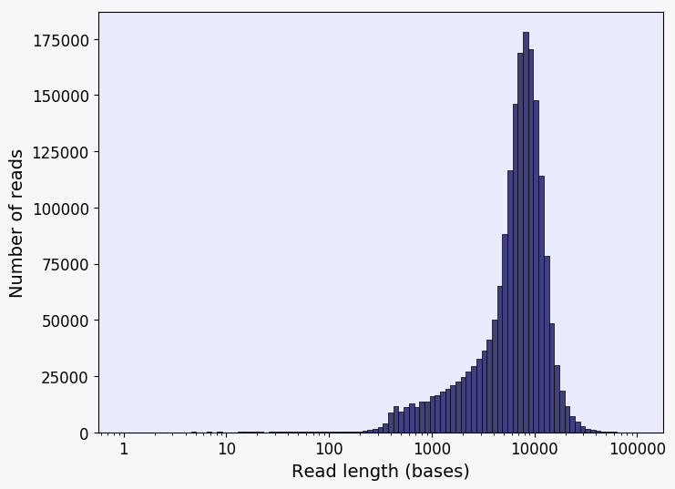
Histogram showing the distribution of read lengths of the long reads from the input sample FASTA file. Ideally, majority of the reads should have lengths more than 1000 bases for reliable SV characterization analysis by NanoVar.
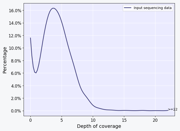
This plot shows the estimated depth of coverage across the reference genome by mapped long reads of the input sample. The curve is estimated from calculating the read depth across 10000 random points in the reference genome. Ideally, the plot should look similar to the one shown here or has a curve that is shifted more toward the right. For comprehensive SV discovery, the peak of the curve should be more than or close to 4X depth of coverage as shown in the plot here or 8X depth for better resolution of heterozygous SVs.